Documentation on nef.x
nef.x is a package to analyze nef partitions of a reflexive polytope. Such nef partitions determine complete intersections of Calabi-Yau type in toric varieties of, in principle, arbitrary codimension. Given a reflexive polytope in terms of a combined weight system or a list of points the main objective of the program is to determine the nef partitions and the Hodge numbers of the corresponding Calabi-Yau varieties. Further features include the calculation of the corresponding reflexive Gorenstein cones as well as information about the fibration structure.
The corresponding routines are listed in the header file Nef.h.
Contents |
Nef partitions and reflexive Gorenstein cones
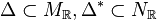
Consider a dual pair of d-dimensional reflexive polytopes
 . A
partition
. A
partition  of the set of vertices of
Δ * into disjoint subsets
of the set of vertices of
Δ * into disjoint subsets  is called a
nef partition of length r if there exist r integral upper convex
Σ(Δ * )-piecewise linear support functions
is called a
nef partition of length r if there exist r integral upper convex
Σ(Δ * )-piecewise linear support functions
 ,
,  such that
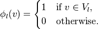
Each ϕl corresponds to a divisor 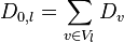 on the toric variety
  associated to Δ * , and
the intersection of all these divisors
associated to Δ * , and
the intersection of all these divisors
defines a family  of Calabi-Yau complete
intersections of codimension r.
of Calabi-Yau complete
intersections of codimension r.
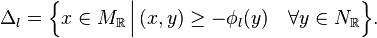
Moreover, each ϕl corresponds to a lattice polyhedron Δl defined as
The sum of the functions ϕl is equal to the
support function of the anticanonical divisor  and, therefore, the
corresponding Minkowski sum is
and, therefore, the
corresponding Minkowski sum is  .
Moreover, the knowledge of the decomposition
is equivalent to that of the set of supporting polyhedra
.
Moreover, the knowledge of the decomposition
is equivalent to that of the set of supporting polyhedra
 , and therefore this data is
often also called a nef partition.
, and therefore this data is
often also called a nef partition.
For a given nef partition Π(Δ) the polytopes (The brackets  denote the convex hull.)
define again a nef partition
 such that the Minkowski
sum
such that the Minkowski
sum  is a reflexive
polytope. Then, its dual
is a reflexive
polytope. Then, its dual  is also reflexive, and
 is called the dual nef partition. This is the
combinatorial manifestation of mirror symmetry in terms of dual
pairs of nef partitions of Δ * and , which we
summarize in the following diagram
is called the dual nef partition. This is the
combinatorial manifestation of mirror symmetry in terms of dual
pairs of nef partitions of Δ * and , which we
summarize in the following diagram
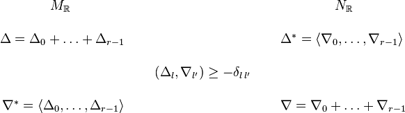
In the horizontal direction, we have the duality between the lattices
M and N and mirror symmetry goes from the upper right to the lower
left. The complete intersections and  associated to the dual nef partitions are then
mirror Calabi-Yau varieties.
associated to the dual nef partitions are then
mirror Calabi-Yau varieties.
There are two constructions to build new nef partitions from old ones:
projections and direct products.
Given a nef partition
where one of the subsets Vl, say V0,
consists of a single vertex v, the nef condition implies that the
projection  of Δ * along v is
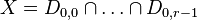
reflexive. Moreover,the Calabi-Yau complete
intersection X is given by
of Δ * along v is
reflexive. Moreover,the Calabi-Yau complete
intersection X is given by  with
with  . Since D can only intersect the toric divisors that
correspond to points bounding the reflexive projection along v, the
variety X is isomorphic to the variety
. Since D can only intersect the toric divisors that
correspond to points bounding the reflexive projection along v, the
variety X is isomorphic to the variety  , where
  is obtained from the
projection . In hep-th/0410018 such nef partitions
were called trivial.
In nef.x they are labeled by P for projection,
see -P.
is obtained from the
projection . In hep-th/0410018 such nef partitions
were called trivial.
In nef.x they are labeled by P for projection,
see -P.
Suppose we are given two lattices M(1),M(2) and two reflexive polytopes
 ,
,  such that (Δ(1)) * and (Δ(2)) * admit
nef partitions
such that (Δ(1)) * and (Δ(2)) * admit
nef partitions  and
and
 , respectively.
Then
, respectively.
Then  is
reflexive with respect to
is
reflexive with respect to  and dual to Δ *
whose set of vertices V is
and dual to Δ *
whose set of vertices V is  .
V admits a nef partition induced from the
nef partitions V(1) and V(2). Such a nef partition is
called a direct product since the corresponding Calabi-Yau complete
intersection X is a direct product
.
V admits a nef partition induced from the
nef partitions V(1) and V(2). Such a nef partition is
called a direct product since the corresponding Calabi-Yau complete
intersection X is a direct product  in
in  .
.
One can reformulate the duality of nef partitions in terms of
reflexive Gorenstein cones as follows. We extend the lattices M and
N to  and
and  and set
  .
.
A  -dimensional rational polyhedral cone C
in
-dimensional rational polyhedral cone C
in  is called Gorenstein
if
is called Gorenstein
if  , there
exists an element
, there
exists an element  such that
  for any nonzero
  , and all
vertices of the
, and all
vertices of the  -dimensional convex polytope

belong to
 .
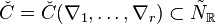
The polytope Δ(C) is called
the support of C.
Conversely, any -dimensional lattice polytope Λ
determines a -dimensional Gorenstein cone C(Λ) as the cone
over Λ with apex at lattice distance 1 from the hyperplane carrying Λ;
obviously Δ(C(Λ)) = Λ.
For any
.
The polytope Δ(C) is called
the support of C.
Conversely, any -dimensional lattice polytope Λ
determines a -dimensional Gorenstein cone C(Λ) as the cone
over Λ with apex at lattice distance 1 from the hyperplane carrying Λ;
obviously Δ(C(Λ)) = Λ.
For any  , we define the degree of m as
  .
.
A Gorenstein cone C is called reflexive if the dual cone

is also Gorenstein, i.e., there exists  such that
  for all
  , and all vertices of the
support
, and all vertices of the
support
 belong to
  . We will call the integer
  the index of C (or
  ).
).
Any
nef partition
of length r of a reflexive polytope Δ
determines
a -dimensional
dual pair of reflexive Gorenstein cones
 ,
,
 of index r by


There are, however, reflexive Gorenstein cones that do not come from nef partitions.
A reflexive Gorenstein cone admits a representation in terms of the
points of the underlying reflexive polytope as follows. Given a
point
 , the
corresponding point
, the
corresponding point  is given as

where ϕl is the support function defined above.
To see that the two descriptions of are equivalent, note
that both correspond to a cone whose support has vertices

where {ei} is the standard basis of  , i(k) is the number
such that
, i(k) is the number
such that  and 0N is the origin in the N-lattice.
The Hodge numbers of a Calabi-Yau manifold X defined by means of a
nef partition depend only on the structure of
the corresponding reflexive Gorenstein cone in a manner described in
math/0103214 or alg-geom/9509009.
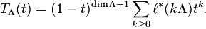
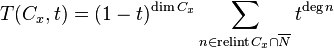
The corresponding formulas rely heavily on the counting of lattice points.
For any lattice polytope Λ let us denote by  the number
of lattice points of Λ and by
the number
of lattice points of Λ and by  the number of lattice
points in the interior of Λ.
It can be shown that
the number of lattice
points in the interior of Λ.
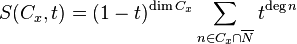
It can be shown that
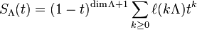
is a polynomial of degree  ;
SΛ(t) is called the Ehrhart polynomial of Λ.
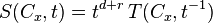
Similarly one can define a polynomial
;
SΛ(t) is called the Ehrhart polynomial of Λ.
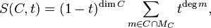
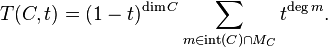
Similarly one can define a polynomial
In terms of a Gorenstein cone C over Λ, with underlying lattice MC, S and T can be written as
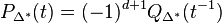
The two polynomials satisfy a relation which is a consequence of Serre duality,
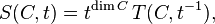
which provides a stringent test on any results involving lattice point counting. For the computation of Hodge numbers, the S- and T- polynomials for all the faces of C(Δ) as well as a polynomial called B, which is related to the poset structure of C(Δ), are required.
Standard output
In this subsection we will explain in detail how to interpret the output of nef.x when called without any options.
The standard output slightly depends on whether the reflexive polytope is input as a combined weight system or as a collection of points. If the polytope was entered as a collection of points, the first line of the output takes the following form:
M:# # N:# # codim=# #part=#
Note that the input polytope is interpreted as  unless the option -N is used,
while any output of a polytope in matrix format refers to its dual
unless the option -N is used,
while any output of a polytope in matrix format refers to its dual
 except for the option -y.
If the input is a CWS, the line starts with the CWS repeated before the
symbol M.
except for the option -y.
If the input is a CWS, the line starts with the CWS repeated before the
symbol M.
# M:# # N:# # codim=# #part=#
where the first # stands for the sequence of numbers describing the
CWS.
The two numbers # after
M correspond to the numbers of
lattice points and vertices of and the
numbers # after N correspond to the numbers of lattice
points and vertices of ,
respectively.
The number r in
codim=r is the length of the nef partition, i.e. the codimension
of the corresponding Calabi-Yau complete intersection. The
default value is 2, otherwise it is specified by the option -c*. The number n in #part=n is the number of all the nef partitions that nef.x
has found, up to symmetries of the underlying lattice. If the
symmetries of the underlying lattice should not be taken into account,
use the option -s.
The subsequent lines contain the information about the various nef partitions. Note that the standard output suppresses the output of nef partitions which are equivalent under symmetries of the CWS. If the codimension is 2 the output line containing the information on a particular nef partition takes the following form:
H:# [#] P:# V:# # #sec #cpu
The numbers # after H: are the Hodge numbers  , where d is the dimension of the Calabi-Yau
manifold X.
, where d is the dimension of the Calabi-Yau
manifold X.
The number $ in the square brackets [#] is the Euler
number of X. If  for some
  the
Calabi-Yau manifold factorizes. See the option -D for this case. In any case, the full Hodge
diamond is displayed with the option -H.
the
Calabi-Yau manifold factorizes. See the option -D for this case. In any case, the full Hodge
diamond is displayed with the option -H.
The number # after P: is a counter specifying the nef partition. It runs from 0 to n - 1. Note that nef partitions corresponding to direct products and projections to nef partitions of lower length are omitted by default. To display them use the options -D, -Q for direct products and -P for projections.
The sequence of numbers # separated by a single space after V: corresponds to the vertices that belong to the first part V0 of the nef partition. Note that the vertices are counted starting from 0. These numbers only make sense if the options -n, -Lv or -Lp are used. The vertices that belong to the second part <maht>V_1</math> of the nef partition are not displayed, since they are simply the remaining ones. If the polytope entered also has points that are not vertices or if the option -Lv is used, then the second sequence of numbers # that is separated from the first sequence by two spaces corresponds to the non-vertex points that belong to the first part V0. For representations of the nef partition in terms of the Gorenstein cone see the option -g*.
The number # before sec indicates the time that was needed to compute this partition. The number # before cpu indicates the number of CPU seconds that were needed to compute the Hodge numbers. For determining the nef partitions without computing the Hodge numbers see the option -p.
If the length r is bigger than 2 the lines containing the information about the various nef partitions take the following form:
H:# [#] P:# V0:# # V1:# # ... V(r-2):# # #sec #cpu
Now, there are r - 1 expressions of the form Vi:# #, where i runs from 0 to r - 2 each representing a part Vi of the nef partition. The points and vertices in each Vi are listed in the same order as in the codimension two case.
The final line of the output always takes the following form:
np=# d:# p:# #sec #cpu
The numbers # after d:, p:, np= are the numbers of nef partitions which are direct products, projections, and neither of the two, respectively. The total of the three numbers adds up to n, the total number of nef partitions as indicated in the first line after #part=. The number # before sec indicates the time that was needed to compute all the partitions. The number # before cpu indicates the number of CPU seconds that were needed to compute the Hodge numbers of all the nef partitions.
The following example illustrates the standard output of nef.x. We
consider complete intersections of codimension 2 in
 discussed in arXiv:0704.0449[hep-th]
. Let
discussed in arXiv:0704.0449[hep-th]
. Let  be the standard basis of
  .
We define the polytope
.
We define the polytope  by the vertices
 given by
v0 = e1,v1 = e2,v2 = − e1 − e2,v3 = e3,v4 = − e3,v5 = e4,v6 = e5,v7 = − e4 − e5.
By elementary toric geometry, we see that  and the combined
weight system can be read off from the linear relations
and the combined
weight system can be read off from the linear relations
v0 + v1 + v2 = 0,v3 + v4 = 0,v5 + v6 + v7 = 0.
First, we enter the polytope by giving this combined weight system
palp$ nef.x
Degrees and weights  `d1 w11 w12 ... d2 w21 w22 ...'
  or `#lines #colums' (= `PolyDim #Points' or `#Points PolyDim'):
3 1 1 1 0 0 0 0 0  2 0 0 0 1 1 0 0 0  3 0 0 0 0 0 1 1 1
3 1 1 1 0 0 0 0 0  2 0 0 0 1 1 0 0 0  3 0 0 0 0 0 1 1 1
M:300 18 N:9 8  codim=2 #part=15
H:19 19 [0] P:0 V:2 4 6 7       1sec  0cpu
H:9 27 [-36] P:2 V:3 4 6 7       1sec  0cpu
H:3 51 [-96] P:3 V:3 5 6 7       1sec  1cpu
H:3 75 [-144] P:4 V:3 6 7       1sec  0cpu
H:3 51 [-96] P:6 V:4 5 6 7       2sec  1cpu
H:3 51 [-96] P:7 V:4 5 6       1sec  1cpu
H:6 51 [-90] P:8 V:4 6 7       1sec  1cpu
H:3 75 [-144] P:9 V:4 6       1sec  1cpu
H:3 60 [-114] P:10 V:5 6 7       2sec  1cpu
H:3 69 [-132] P:11 V:5 6       1sec  1cpu
H:3 75 [-144] P:12 V:6 7       1sec  0cpu
np=11 d:2 p:2    0sec     0cpu
Equivalently, we can use the option -N and enter the points of
the polytope Δ * of the normal fan of
:
palp$ nef.x -N
Degrees and weights  `d1 w11 w12 ... d2 w21 w22 ...'
  or `#lines #colums' (= `PolyDim #Points' or `#Points PolyDim'):
5 8
Type the 40 coordinates as dim=5 lines with #pts=8 colums:
 1  0 -1  0  0  0  0  0
 0  1 -1  0  0  0  0  0
 0  0  0  1 -1  0  0  0
 0  0  0  0  0  1  0 -1
 0  0  0  0  0  0  1 -1
M:300 18 N:9 8  codim=2 #part=15
H:3 51 [-96] P:0 V:2 3 4 7       1sec  1cpu
H:3 51 [-96] P:1 V:2 4 6 7       2sec  1cpu
H:3 60 [-114] P:2 V:2 4 7       2sec  1cpu
H:3 51 [-96] P:3 V:2 6 7       1sec  1cpu
H:3 69 [-132] P:4 V:2 7       1sec  1cpu
H:9 27 [-36] P:5 V:3 4 6 7       1sec  0cpu
H:3 75 [-144] P:6 V:3 4 7       0sec  0cpu
H:19 19 [0] P:8 V:4 5 6 7       1sec  0cpu
H:6 51 [-90] P:9 V:4 6 7       1sec  1cpu
H:3 75 [-144] P:10 V:4 7       1sec  0cpu
H:3 75 [-144] P:13 V:6 7       1sec  1cpu
np=11 d:2 p:2    0sec     0cpu
Note that both the points and the nef partitions are given in different orders.
The polytope  has 9 points, 8 vertices
and the interior point, while the dual polytope
has 9 points, 8 vertices
and the interior point, while the dual polytope  has 300 points, 18 of which are vertices. The codimension
is 2 and there are 15 nef partitions.
There are 11 nef partitions listed, furthermore there are 2 nef partitions which are direct products, and 2 which are projections.
According to the output the nef partitions e.g. 0 and 8 are given as follows (with the Hodge numbers and the Euler number of the corresponding Calabi-Yau 3-fold X):
has 300 points, 18 of which are vertices. The codimension
is 2 and there are 15 nef partitions.
There are 11 nef partitions listed, furthermore there are 2 nef partitions which are direct products, and 2 which are projections.
According to the output the nef partitions e.g. 0 and 8 are given as follows (with the Hodge numbers and the Euler number of the corresponding Calabi-Yau 3-fold X):


Global parameters and limitations
If the dimension of the polytope or the codimension of the nef partition are large, certain global variables in the header files Global.h and Nef.h may need to be modified. This depends very much on the problem to be treated by nef.x as well as on the CPU and the operating system of the computer nef.x is running on. Here we give a particularly nasty example:
palp$ nef.x -Lp -N -c6 -P
Degrees and weights  `d1 w11 w12 ... d2 w21 w22 ...'
  or `#lines #columns' (= `PolyDim #Points' or `#Points PolyDim'):
7 9
Please increase POLY_Dmax to at least 12 = 7 + 6 - 1
(nef.x requires POLY_Dmax >= dim N + codim - 1)
This means that in Global.h we need to set POLY_Dmax to at least 12:
#define POLY_Dmax 12 /* max dim of polytope */
After recompiling PALP we get further but not far enough:
palp$ ./nef.x -Lp -N -c6 -P
Degrees and weights  `d1 w11 w12 ... d2 w21 w22 ...'
  or `#lines #columns' (= `PolyDim #Points' or `#Points PolyDim'):
7 9
Type the 63 coordinates as dim=7 lines with #pts=9 columns:
 1  0  0  0  0 -1  0  0 -1
 0  1  0  0  0 -1  0  0 -1
 0  0  1  0  0 -1  0  0 -1
 0  0  0  1  0 -1  0  0  0
 0  0  0  0  1 -1  0  0  0
 0  0  0  0  0  0  1  0 -1
 0  0  0  0  0  0  0  1 -1
M:5214 12 N:10 9  codim=6 #part=1
7 10  Points of Poly in N-Lattice:
    1    0    0    0    0   -1    0    0   -1    0
    0    1    0    0    0   -1    0    0   -1    0
    0    0    1    0    0   -1    0    0   -1    0
    0    0    0    1    0   -1    0    0    0    0
    0    0    0    0    1   -1    0    0    0    0
    0    0    0    0    0    0    1    0   -1    0
    0    0    0    0    0    0    0    1   -1    0
--------------------------------------------------
    1    1    1    1    1    1    0    0    0  d=6  codim=2
    1    1    1    0    0    0    1    1    1  d=6  codim=2
nef.x: Vertex.c:613: Finish_Find_Equations:
                     Assertion `_V->nv<64' failed.
Aborted
This can be remedied by adjusting the global variable VERT_Nmax in Global.h as follows (it should not be too large):
#define VERT_Nmax 128 /* !! use optimal value !! */
After recompilation it works for a while. Then the following error occurs
Unable to alloc space for _BL
This means that the program has run out of memory.
Help screen
The help screen for nef.x is:
palp$ ./nef.x -h

This is './nef.x':  calculate Hodge numbers of nef-partitions
Usage:   ./nef.x <Options>

Options: -h        prints this information
         -f or -   use as filter; otherwise parameters denote I/O files
         -N        input is in N-lattice (default is M)
         -H        gives full list of Hodge numbers
         -Lv       prints L vector of Vertices (in N-lattice)
         -Lp       prints L vector of Points (in N-lattice)
         -p        prints only partitions, no Hodge numbers
         -D        calculates also direct products
         -P        calculates also projections
         -t        full time info
         -cCODIM   codimension (default = 2)
         -Fcodim   fibrations up to codim (default = 2)
         -y        prints poly/CWS in M lattice if it has nef-partitions
         -S        information about #points calculated in S-Poly
         -T        checks Serre-duality
         -s        don't remove symmetric nef-partitions
         -n        prints polytope only if it has nef-partitions
         -v        prints vertices and #points of input polytope in one
                   line; with -u, -l the output is limited by #points:
             -uPOINTS  ... upper limit of #points (default = POINT_Nmax)
             -lPOINTS  ... lower limit of #points (default = 0)
         -m        starts with [d  w1 w2 ... wk d=d_1 d_2 (Minkowski sum)
         -R        prints vertices of input if not reflexive
         -V        prints vertices of N-lattice polytope
         -Q        only direct products (up to lattice Quotient)
         -gNUMBER  prints points of Gorenstein polytope in N-lattice
         -dNUMBER  prints points of Gorenstein polytope in M-lattice
               if NUMBER = 0 ... no            0/1 info
               if NUMBER = 1 ... no redundant  0/1 info (=default)
               if NUMBER = 2 ... full          0/1 info
         -G        Gorenstein cone: input <-> support polytope
The options in detail
-N
The option -N interprets the input polytope in the lattice N. The default lattice for the input polytope, however, is the lattice M. The default lattice for the output polytope is the lattice N.
The following example of a complete intersection of degree (2,2) in  illustrates the difference. In order to point out the difference we display the points in the two lattices with the option -Lv.
palp$ nef.x -Lv
Degrees and weights  `d1 w11 w12 ... d2 w21 w22 ...'
  or `#lines #colums' (= `PolyDim #Points' or `#Points PolyDim'):
3 4
Type the 12 coordinates as dim=3 lines with #pts=4 colums:
   -1    0    0    1
   -1    0    1    0
   -1    1    0    0
M:5 4 N:35 4  codim=2 #part=0
3 4 Vertices in N-lattice:
   -1   -1   -1    3
   -1   -1    3   -1
   -1    3   -1   -1
--------------------
    1    1    1    1  d=4  codim=0
np=0 d:0 p:0    0sec     0cpu
Without the option -N, the output polytope is the dual of the input polytope with 35 points and no nef partition.
palp$ nef.x -Lv -N
Degrees and weights  `d1 w11 w12 ... d2 w21 w22 ...'
  or `#lines #colums' (= `PolyDim #Points' or `#Points PolyDim'):
3 4
Type the 12 coordinates as dim=3 lines with #pts=4 colums:
   -1    0    0    1
   -1    0    1    0
   -1    1    0    0
M:35 4 N:5 4  codim=2 #part=2
3 4 Vertices in N-lattice:
   -1    0    0    1
   -1    0    1    0
   -1    1    0    0
--------------------
    1    1    1    1  d=4  codim=0
H:[0] P:0 V:2 3   (2 2)     0sec  0cpu
np=1 d:0 p:1    0sec     0cpu
With the option -N, the output polytope is the same as input polytope with 4 points and the expected nef partition corresponding to the complete intersection of degree (2,2) in . Note that the order of the points in the output is the same as in the input. This last feature is the main advantage of the option -N. To see this we consider the example used in the description of the standard output, the complete intersections of codimension 2 in discussed in arXiv:0704.0449[hep-th].
palp$ nef.x -Lv
Degrees and weights  `d1 w11 w12 ... d2 w21 w22 ...'
  or `#lines #colums' (= `PolyDim #Points' or `#Points PolyDim'):
3 1 1 1 0 0 0 0 0  2 0 0 0 1 1 0 0 0  3 0 0 0 0 0 1 1 1
3 1 1 1 0 0 0 0 0  2 0 0 0 1 1 0 0 0  3 0 0 0 0 0 1 1 1 M:300 18 N:9 8  codim=2 #part=15
5 8 Vertices in N-lattice:
    0    0    0    0    1    0   -1    0
    0    0    1    0    0    0   -1    0
    0    0    0    1    0    0    0   -1
   -1    0    0    0    0    1    0    0
   -1    1    0    0    0    0    0    0
----------------------------------------
    1    1    0    0    0    1    0    0  d=3  codim=3
    0    0    1    0    1    0    1    0  d=3  codim=3
    0    0    0    1    0    0    0    1  d=2  codim=4
H:19 19 [0] P:0 V:2 4 6 7   (0 3) (3 0) (1 1)     1sec  0cpu
H:9 27 [-36] P:2 V:3 4 6 7   (0 3) (2 1) (2 0)     0sec  0cpu
H:3 51 [-96] P:3 V:3 5 6 7   (1 2) (1 2) (2 0)     1sec  0cpu
H:3 75 [-144] P:4 V:3 6 7   (0 3) (1 2) (2 0)     0sec  0cpu
H:3 51 [-96] P:6 V:4 5 6 7   (1 2) (2 1) (1 1)     2sec  1cpu
H:3 51 [-96] P:7 V:4 5 6   (1 2) (2 1) (0 2)     1sec  0cpu
H:6 51 [-90] P:8 V:4 6 7   (0 3) (2 1) (1 1)     1sec  0cpu
H:3 75 [-144] P:9 V:4 6   (0 3) (2 1) (0 2)     0sec  0cpu
H:3 60 [-114] P:10 V:5 6 7   (1 2) (1 2) (1 1)     2sec  1cpu
H:3 69 [-132] P:11 V:5 6   (1 2) (1 2) (0 2)     1sec  0cpu
H:3 75 [-144] P:12 V:6 7   (0 3) (1 2) (1 1)     0sec  0cpu
np=11 d:2 p:2    0sec     0cpu
Note that the basis chosen does not respect the order given by the combined weight system that was entered. E.g. the weight vector 2 0 0 0 1 1 0 0 0 has changed to the linear relation 0 0 0 1 0 0 0 1 d=2 where the 0's and 1's are in a different order. This can be overcome using the option -N. We choose a basis for the lattice such that the vertices of the polytope satisfy the desired combined weight system 3 1 1 1 0 0 0 0 0 2 0 0 0 1 1 0 0 0 3 0 0 0 0 0 1 1 1:
palp$ nef.x -N -Lv
Degrees and weights  `d1 w11 w12 ... d2 w21 w22 ...'
  or `#lines #colums' (= `PolyDim #Points' or `#Points PolyDim'):
5 8
Type the 40 coordinates as dim=5 lines with #pts=8 colums:
 1  0 -1  0  0  0  0  0
 0  1 -1  0  0  0  0  0
 0  0  0  1 -1  0  0  0
 0  0  0  0  0  1  0 -1
 0  0  0  0  0  0  1 -1
M:300 18 N:9 8  codim=2 #part=15
5 8 Vertices in N-lattice:
    1    0   -1    0    0    0    0    0
    0    1   -1    0    0    0    0    0
    0    0    0    1   -1    0    0    0
    0    0    0    0    0    1    0   -1
    0    0    0    0    0    0    1   -1
----------------------------------------
    1    1    1    0    0    0    0    0  d=3  codim=3
    0    0    0    1    1    0    0    0  d=2  codim=4
    0    0    0    0    0    1    1    1  d=3  codim=3
H:3 51 [-96] P:0 V:2 3 4 7   (1 2) (2 0) (1 2)     1sec  0cpu
H:3 51 [-96] P:1 V:2 4 6 7   (1 2) (1 1) (2 1)     1sec  1cpu
H:3 60 [-114] P:2 V:2 4 7   (1 2) (1 1) (1 2)     2sec  1cpu
H:3 51 [-96] P:3 V:2 6 7   (1 2) (0 2) (2 1)     1sec  0cpu
H:3 69 [-132] P:4 V:2 7   (1 2) (0 2) (1 2)     0sec  0cpu
H:9 27 [-36] P:5 V:3 4 6 7   (0 3) (2 0) (2 1)     1sec  0cpu
H:3 75 [-144] P:6 V:3 4 7   (0 3) (2 0) (1 2)     0sec  0cpu
H:19 19 [0] P:8 V:4 5 6 7   (0 3) (1 1) (3 0)     1sec  0cpu
H:6 51 [-90] P:9 V:4 6 7   (0 3) (1 1) (2 1)     1sec  0cpu
H:3 75 [-144] P:10 V:4 7   (0 3) (1 1) (1 2)     0sec  0cpu
H:3 75 [-144] P:13 V:6 7   (0 3) (0 2) (2 1)     1sec  0cpu
np=11 d:2 p:2    0sec     0cpu
The order of the vertices being unchanged, the linear relations agree with the desired combined weight system.
-H
The option -H replaces the output lines starting with H: with the full Hodge diamond of the corresponding partition. Note that the information about the nef partition is omitted. The following example of codimension 2 complete intersections in  illustrates this option
palp$ nef.x -H
Degrees and weights  `d1 w11 w12 ... d2 w21 w22 ...'
  or `#lines #colums' (= `PolyDim #Points' or `#Points PolyDim'):
7 1 1 1 1 1 1 1
7 1 1 1 1 1 1 1 M:1716 7 N:8 7  codim=2 #part=3


                                    h 0 0

                               h 1 0      h 0 1

                          h 2 0      h 1 1      h 0 2

                     h 3 0      h 2 1      h 1 2      h 0 3

                h 4 0      h 3 1      h 2 2      h 1 3      h 0 4

                     h 4 1      h 3 2      h 2 3      h 1 4

                          h 4 2      h 3 3      h 2 4

                               h 4 3      h 3 4

                                    h 4 4


                                       1

                                  0         0

                             0         1         0

                        0         0         0         0

                   1       237       996       237         1

                        0         0         0         0

                             0         1         0

                                  0         0

                                       1

     16sec  15cpu


                                    h 0 0

                               h 1 0      h 0 1

                          h 2 0      h 1 1      h 0 2

                     h 3 0      h 2 1      h 1 2      h 0 3

                h 4 0      h 3 1      h 2 2      h 1 3      h 0 4

                     h 4 1      h 3 2      h 2 3      h 1 4

                          h 4 2      h 3 3      h 2 4

                               h 4 3      h 3 4

                                    h 4 4


                                       1

                                  0         0

                             0         1         0

                        0         0         0         0

                   1       356      1472       356         1

                        0         0         0         0

                             0         1         0

                                  0         0

                                       1

     42sec  41cpu
np=2 d:0 p:1    0sec     0cpu
-Lv
The option -Lv prints the vertices of the output polytope and the linear relations among them in addition to the standard output. If only the vertices should be printed see the option -V. The output takes the following form: The first part before the dashed line is
D n Vertices in N-lattice:
    #    #      ...      #    #

    .    .      ...      .    .
    .    .      ...      .    .
    .    .      ...      .    .

    #    #      ...      #    #
The first line says that the vertices of the polytope in the lattice  are given by the subsequent
  lines with
  entries. The means that the polytope has dimension and is given by vertices which are the columns of the subsequent
  array of numbers #. Note that an arbitrary basis of
  will be chosen.
Below the dashed line the linear relations among these vertices are indicated as follows: Let  denote the vertices corresponding to the columns above the dashed line. For each linear relation among the vertices
  given by
 ,
,
denote its degree by
 .
.
The vertices with non-zero  span a reflexive subpolytope of codimension
  . This is very useful in conjunction with the option -F*.
For each linearly independent linear relation there is a line in the output of the following form:
l_0 l_1 ... l_{n-1} d=l codim=c
In other words, these lines give a basis of the vector space of linear relations among the vertices. The basis is completely fixed by the order of the vertices, and the conditions that each vector, i.e. each linear relation is positive and primitive. To suppress these lines see the option -V.
Moreover, the output lines containing the information about the nef-partitions get additional data besides the standard output. This data are the degrees of the parts of the nef-partition with respect to the linear relations. Consider a codimension  nef-partition defined by collections of vertices
  such that every vertex is a member of some collection
  . The (multi)degree of the nef-partition
  with respect to the linear relation is the vector
  where
where
Note that  , the degree of the linear relation. The degrees are the degrees of the polynomials defining the complete intersection. If the codimension is 2 the output lines describing the nef-partitions take the following form
H:# [#] P:# V:# # (d10 d11) ... (dn0 dn1) #sec #cpu
or if the codimension is bigger than 2
H:# [#] P:# V0:# # V1:# # ... V(r-2):# # (d10 ... d1(r-1)) ... (dn0 ... dn(r-1)) #sec #cpu
The additional data is (d10 d11) ... (dn0 dn1) and (d10 ... d1(r-1)) ... (dn0 ... dn(r-1)), respectively, where n is the number of linearly independent linear relations. If  are the degrees with respect to the i-th linear relation, then di0 =
  , ..., di(r-1) =
  .
.
The following example of a codimension 2 complete intersection taken from arXiv:hep-th/0410018v2 illustrates this option
palp$ nef.x -Lv
Degrees and weights  `d1 w11 w12 ... d2 w21 w22 ...'
  or `#lines #colums' (= `PolyDim #Points' or `#Points PolyDim'):
5 1 1 1 1 1 0 0  4 0 0 0 1 1 1 1
5 1 1 1 1 1 0 0  4 0 0 0 1 1 1 1 M:378 12 N:8 7  codim=2 #part=8
5 7 Vertices in N-lattice:
    0   -1    0    1    0    0    0
    0   -1    1    0    0    0    0
   -1    0    0    0    0    0    1
   -1    1    0    0    1    0    0
   -1    1    0    0    0    1    0
-----------------------------------
    1    1    1    1    0    0    1  d=5  codim=1
    1    0    0    0    1    1    1  d=4  codim=2
H:2 64 [-124] P:0 V:0 6   (2 3) (2 2)     1sec  0cpu
H:2 64 [-124] P:1 V:0 1 6   (3 2) (2 2)     1sec  0cpu
H:2 74 [-144] P:2 V:2 3 5   (2 3) (1 3)     1sec  0cpu
H:2 64 [-124] P:3 V:3 5 6   (2 3) (2 2)     1sec  0cpu
H:2 86 [-168] P:4 V:3 5   (1 4) (1 3)     1sec  1cpu
H:2 74 [-144] P:5 V:3 6   (2 3) (1 3)     1sec  0cpu
np=6 d:0 p:2    0sec     0cpu
The line 5 7 Vertices in N-lattice: says that the polytope has dimension 5 and is given by 7 vertices  .
Let be the standard basis of . From the columns of the subsequent 5 by 7 array of numbers, we read off that the 7 vertices are
.
Let be the standard basis of . From the columns of the subsequent 5 by 7 array of numbers, we read off that the 7 vertices are
 .
.
Note that an arbitrary basis has been chosen. There are two linearly independent linear relations:
 .
.
The first of these linear relations has degree 5, the second has degree 4. The corresponding subpolytopes have codimension 1 and 2, respectively. The nef-partitions and their degrees are then as follows:


-Lp
The option -Lp prints the points of the N-lattice polytope and the linear relations among them. The output has the same structure as for the option -Lv. The points are ordered such that first the vertices are listed, then the points which are not vertices and finally the origin. Note that there will be extra relations including the points which are not vertices.
Example: Complete intersection Calabi-Yau fourfold of codimension two discussed in arXiv:0912.3524. Important: in Global.h set POLY_Dmax=7 or higher and recompile! See Global parameters and limitations.
palp$ nef.x -Lp
Degrees and weights  `d1 w11 w12 ... d2 w21 w22 ...'
  or `#lines #columns' (= `PolyDim #Points' or `#Points PolyDim'):
6 3 2 1 0 0 0 0 0 0 0 0  13 6 4 0 1 0 0 0 0 0 1 1  7 3 2 0 0 1 0 0 0 0 1 0  8 3 2 0 0 0 1 0 0 1 1 0  15 6 4 0 0 0 0 1 1 1 1 1
6 3 2 1 0 0 0 0 0 0 0 0  13 6 4 0 1 0 0 0 0 0 1 1  7 3 2 0 0 1 0 0 0 0 1 0  8 3 2 0 0 0 1 0 0 1 1 0  15 6 4 0 0 0 0 1 1 1 1 1 M:4738 39 N:15 11  codim=2 #part=11
6 15  Points of Poly in N-Lattice:
    0    0   -2    3    0    0    0    0    0    0    0   -1    2    1    0
    0    2   -1    1    0    0    0    1    1    1    2    0    1    1    0
    0    1   -1    1    0    0    1    1    1    1    2    0    1    1    0
    0    1   -1    1    1    0    0    1    0    1    2    0    1    1    0
    0   -1    0    0    0    1    0   -1   -1    0   -1    0    0    0    0
    1   -1    0    0    0    0    0    0    0    0   -1    0    0    0    0
---------------------------------------------------------------------------
    1    1    6    4    1    1    1    0    0    0    0    0    0    0  d=15  codim=0
    1    0    6    4    0    1    0    0    0    0    1    0    0    0  d=13  codim=2
    0    0    3    2    1    1    0    0    1    0    0    0    0    0  d=8  codim=2
    0    0    3    2    0    1    0    1    0    0    0    0    0    0  d=7  codim=3
    0    0    3    2    0    0    0    0    0    1    0    0    0    0  d=6  codim=4
    0    0    1    1    0    0    0    0    0    0    0    1    0    0  d=3  codim=4
    0    0    2    1    0    0    0    0    0    0    0    0    0    1  d=4  codim=4
    0    0    1    0    0    0    0    0    0    0    0    0    1    0  d=2  codim=5
H:8 0 1113 [6774] P:0 V:0 4 7   (2 13) (1 12) (1 7) (1 6) (0 6) (0 3) (0 4) (0 2)     282sec  281cpu
H:5 0 1115 [6768] P:1 V:0 2 3 5 9  11 12 13   (12 3) (12 1) (6 2) (6 1) (6 0) (3 0) (4 0) (2 0)     162sec  162cpu
H:5 0 1115 [6768] P:2 V:1 5 6 8   (3 12) (1 12) (2 6) (1 6) (0 6) (0 3) (0 4) (0 2)     159sec  158cpu
H:8 0 1113 [6774] P:3 V:1 6 7 8 10   (2 13) (1 12) (1 7) (1 6) (0 6) (0 3) (0 4) (0 2)     228sec  216cpu
H:8 0 1113 [6774] P:4 V:0 1 7 8   (2 13) (1 12) (1 7) (1 6) (0 6) (0 3) (0 4) (0 2)     236sec  234cpu
H:5 0 1115 [6768] P:5 V:0 1 4 7 8   (3 12) (1 12) (2 6) (1 6) (0 6) (0 3) (0 4) (0 2)     183sec  182cpu
H:5 0 1115 [6768] P:6 V:4 5 6   (3 12) (1 12) (2 6) (1 6) (0 6) (0 3) (0 4) (0 2)     221sec  220cpu
H:8 0 1113 [6774] P:7 V:4 6 7 10   (2 13) (1 12) (1 7) (1 6) (0 6) (0 3) (0 4) (0 2)     271sec  265cpu
H:8 0 1113 [6774] P:9 V:5 6   (2 13) (1 12) (1 7) (1 6) (0 6) (0 3) (0 4) (0 2)     282sec  281cpu
H:7 0 958 [5838] P:10 V:6 8   (1 14) (0 13) (1 7) (0 7) (0 6) (0 3) (0 4) (0 2)     272sec  -4023cpu
np=10 d:0 p:1  272sec  -4023cpu
The last four points are not vertices. There are three more linear relations including those points. Compare this to the output of the option -Lv:
palp$ nef.x -Lv
Degrees and weights  `d1 w11 w12 ... d2 w21 w22 ...'
  or `#lines #columns' (= `PolyDim #Points' or `#Points PolyDim'):
6 3 2 1 0 0 0 0 0 0 0 0  13 6 4 0 1 0 0 0 0 0 1 1  7 3 2 0 0 1 0 0 0 0 1 0  8 3 2 0 0 0 1 0 0 1 1 0  15 6 4 0 0 0 0 1 1 1 1 1
6 3 2 1 0 0 0 0 0 0 0 0  13 6 4 0 1 0 0 0 0 0 1 1  7 3 2 0 0 1 0 0 0 0 1 0  8 3 2 0 0 0 1 0 0 1 1 0  15 6 4 0 0 0 0 1 1 1 1 1 M:4738 39 N:15 11  codim=2 #part=11
6 11 Vertices in N-lattice:
    0    0   -2    3    0    0    0    0    0    0    0
    0    2   -1    1    0    0    0    1    1    1    2
    0    1   -1    1    0    0    1    1    1    1    2
    0    1   -1    1    1    0    0    1    0    1    2
    0   -1    0    0    0    1    0   -1   -1    0   -1
    1   -1    0    0    0    0    0    0    0    0   -1
-------------------------------------------------------
    1    1    6    4    1    1    1    0    0    0    0  d=15  codim=0
    1    0    6    4    0    1    0    0    0    0    1  d=13  codim=2
    0    0    3    2    1    1    0    0    1    0    0  d=8  codim=2
    0    0    3    2    0    1    0    1    0    0    0  d=7  codim=3
    0    0    3    2    0    0    0    0    0    1    0  d=6  codim=4
H:8 0 1113 [6774] P:0 V:0 4 7   (2 13) (1 12) (1 7) (1 6) (0 6)     284sec  283cpu
H:5 0 1115 [6768] P:1 V:0 2 3 5 9  11 12 13   (12 3) (12 1) (6 2) (6 1) (6 0)     163sec  163cpu
H:5 0 1115 [6768] P:2 V:1 5 6 8   (3 12) (1 12) (2 6) (1 6) (0 6)     159sec  158cpu
H:8 0 1113 [6774] P:3 V:1 6 7 8 10   (2 13) (1 12) (1 7) (1 6) (0 6)     211sec  210cpu
H:8 0 1113 [6774] P:4 V:0 1 7 8   (2 13) (1 12) (1 7) (1 6) (0 6)     235sec  234cpu
H:5 0 1115 [6768] P:5 V:0 1 4 7 8   (3 12) (1 12) (2 6) (1 6) (0 6)     181sec  180cpu
H:5 0 1115 [6768] P:6 V:4 5 6   (3 12) (1 12) (2 6) (1 6) (0 6)     220sec  220cpu
H:8 0 1113 [6774] P:7 V:4 6 7 10   (2 13) (1 12) (1 7) (1 6) (0 6)     258sec  257cpu
H:8 0 1113 [6774] P:9 V:5 6   (2 13) (1 12) (1 7) (1 6) (0 6)     282sec  281cpu
H:7 0 958 [5838] P:10 V:6 8   (1 14) (0 13) (1 7) (0 7) (0 6)     271sec  -4024cpu
np=10 d:0 p:1  271sec  -4024cpu
-p
Computes the nef partitions without the (time-consuming) calculation of Hodge numbers.
Example: Complete intersection Calabi-Yau fourfold of codimension two discussed in arXiv:0912.3524. Important: in Global.h set POLY_Dmax=7 or higher and recompile! See Global parameters and limitations.
Input with -p:
palp$ nef.x -p
Degrees and weights  `d1 w11 w12 ... d2 w21 w22 ...'
  or `#lines #columns' (= `PolyDim #Points' or `#Points PolyDim'):
6 3 2 1 0 0 0 0 0 0 0 0  13 6 4 0 1 0 0 0 0 0 1 1  7 3 2 0 0 1 0 0 0 0 1 0  8 3 2 0 0 0 1 0 0 1 1 0  15 6 4 0 0 0 0 1 1 1 1 1
6 3 2 1 0 0 0 0 0 0 0 0  13 6 4 0 1 0 0 0 0 0 1 1  7 3 2 0 0 1 0 0 0 0 1 0  8 3 2 0 0 0 1 0 0 1 1 0  15 6 4 0 0 0 0 1 1 1 1 1 M:4738 39 N:15 11  codim=2 #part=11
 P:0 V:0 4 7       0sec  0cpu
 P:1 V:0 2 3 5 9  11 12 13       0sec  0cpu
 P:2 V:1 5 6 8       0sec  0cpu
 P:3 V:1 6 7 8 10       0sec  0cpu
 P:4 V:0 1 7 8       0sec  0cpu
 P:5 V:0 1 4 7 8       0sec  0cpu
 P:6 V:4 5 6       0sec  0cpu
 P:7 V:4 6 7 10       0sec  0cpu
 P:9 V:5 6       0sec  0cpu
 P:10 V:6 8       0sec  0cpu
np=10 d:0 p:1    0sec     0cpu
Input without -p (note the calculation time! (32-bit system)):
palp$ nef.x
Degrees and weights  `d1 w11 w12 ... d2 w21 w22 ...'
  or `#lines #columns' (= `PolyDim #Points' or `#Points PolyDim'):
6 3 2 1 0 0 0 0 0 0 0 0  13 6 4 0 1 0 0 0 0 0 1 1  7 3 2 0 0 1 0 0 0 0 1 0  8 3 2 0 0 0 1 0 0 1 1 0  15 6 4 0 0 0 0 1 1 1 1 1
6 3 2 1 0 0 0 0 0 0 0 0  13 6 4 0 1 0 0 0 0 0 1 1  7 3 2 0 0 1 0 0 0 0 1 0  8 3 2 0 0 0 1 0 0 1 1 0  15 6 4 0 0 0 0 1 1 1 1 1 M:4738 39 N:15 11  codim=2 #part=11
H:8 0 1113 [6774] P:0 V:0 4 7       247sec  246cpu
H:5 0 1115 [6768] P:1 V:0 2 3 5 9  11 12 13       141sec  141cpu
H:5 0 1115 [6768] P:2 V:1 5 6 8       136sec  136cpu
H:8 0 1113 [6774] P:3 V:1 6 7 8 10       183sec  182cpu
H:8 0 1113 [6774] P:4 V:0 1 7 8       203sec  202cpu
H:5 0 1115 [6768] P:5 V:0 1 4 7 8       157sec  156cpu
H:5 0 1115 [6768] P:6 V:4 5 6       190sec  189cpu
H:8 0 1113 [6774] P:7 V:4 6 7 10       226sec  225cpu
H:8 0 1113 [6774] P:9 V:5 6       246sec  246cpu
H:7 0 958 [5838] P:10 V:6 8       236sec  234cpu
np=10 d:0 p:1  236sec   234cpu
-D
This option keeps those nef partitions which are direct products of lower-dimensional nef partitions.
Example: Codimension 2 CICY in 
with option -D:
palp$ nef.x -D
3 1 1 1 0 0 0 3 0 0 0 1 1 1
3 1 1 1 0 0 0  3 0 0 0 1 1 1 M:100 9 N:7 6  codim=2 #part=5
H:4 [0] h1=2 P:0 V:2 3 5   D     0sec  0cpu
H:20 [24] P:1 V:3 4 5       0sec  0cpu
H:20 [24] P:2 V:3 5       0sec  0cpu
H:20 [24] P:3 V:4 5       0sec  0cpu
np=3 d:1 p:1    0sec     0cpu
The last three nef partitions describe a K3 manifold. The first one is a  . The extra output triggered by -D is:
H:4 [0] h1=2 P:0 V:2 3 5 D 0sec 0cpu
h1=2 indicates that the Hodge number  . Furthermore the symbol D indicates that the nef partition is a direct product.
Compare this to the output without the option -D where the first nef partition is not shown:
palp$ nef.x
3 1 1 1 0 0 0 3 0 0 0 1 1 1
3 1 1 1 0 0 0  3 0 0 0 1 1 1 M:100 9 N:7 6  codim=2 #part=5
H:20 [24] P:1 V:3 4 5       0sec  0cpu
H:20 [24] P:2 V:3 5       0sec  0cpu
H:20 [24] P:3 V:4 5       1sec  0cpu
np=3 d:1 p:1    0sec     0cpu
-P
This option also shows nef partitions corresponding to projections. If a nef partition has  elements which only contain one vertex this corresponds to linear equations which set of the homogeneous variables of the toric variety to zero. The corresponding Calabi-Yau manifold can thus be described by a complete intersection of codimension less in a toric variety whose dimension is less.
Example: Complete intersection of codimension 2 in :
palp$ nef.x -P
4 1 1 1 1
4 1 1 1 1 M:35 4 N:5 4  codim=2 #part=2
H:[0] P:0 V:2 3       0sec  0cpu
H:[0] P:1 V:3       0sec  0cpu
np=1 d:0 p:1    0sec     0cpu
Compared to the output without -P there is one additional line:
H:[0] P:1 V:3 0sec 0cpu
Let  be the standard basis of
  . Let
. Let  denote the vertices of the polytope with

The nef-partition P:0 is then as follows
 The part
  only contains the vertex labeled by 3. Therefore the corresponding equation of the complete intersections reads
  . Thus, we are left with a hypersurface of degree 3 in
  , i.e. the cubic curve.
Example: A complete intersection of codimension 6 which is reduced to codimension 3 by projections. We use the option -c* to set the codimension and -p to suppress the calculation of the Hodge numbers. Furthermore we list the vertices using the option -Lv:
palp$ nef.x -P -c6 -p -Lv
Degrees and weights  `d1 w11 w12 ... d2 w21 w22 ...'
  or `#lines #columns' (= `PolyDim #Points' or `#Points PolyDim'):
6 1 1 1 1 1 1 0 0 0 6 1 1 1 0 0 0 1 1 1
6 1 1 1 1 1 1 0 0 0  6 1 1 1 0 0 0 1 1 1 M:5214 12 N:10 9  codim=6 #part=1
7 9 Vertices in N-lattice:
   -1    0    0    1    0    0    0    0    0
   -1    0    1    0    0    0    0    0    0
    0   -1    0    0    0    1    0    0    0
    0   -1    0    0    1    0    0    0    0
   -1    1    0    0    0    0    0    0    1
   -1    1    0    0    0    0    1    0    0
   -1    1    0    0    0    0    0    1    0
---------------------------------------------
    1    1    1    1    1    1    0    0    0  d=6  codim=2
    1    0    1    1    0    0    1    1    1  d=6  codim=2
 P:0 V0:0  V1:2  V2:3  V3:4 7  V4:5 8   (1 1 1 1 1 1) (1 1 1 1 1 1)     0sec  0cpu
np=0 d:0 p:1    0sec     0cpu
The output shows that three elements of the nef partition contain only one vertex:
P:0 V0:0 V1:2 V2:3 V3:4 7 V4:5 8 0sec 0cpu
Therefore the variables associated to the vertices labeled by 0,2 and 3 can be set to zero and we are left with a complete intersection of codimension 3 in .
DP: If there is a nef-partition such that the (dual) nef-partition in the M-lattice has a summand with only one vertex, then a DP is displayed in the output (probably, meaning something like dual projection). See the end of -n for such an example. These two properties are not directly related, P does not necessarily imply DP or vice versa.
-t
The option -t gives detailed information about the calculation times of the Hodge numbers. The Hodge numbers of a complete intersection are generated by the so called stringy E-function introduced by Batyrev and Borisov in alg-geom/9509009. The combinatorial construction of the E-function involves the construction of a B-polynomial and an S-polynomial defined in alg-geom/9509009. The option -t returns the accumulated computing times of the respective polynomials.
Example: Complete intersection Calabi-Yau fourfold discussed in arXiv:0908.1784. Important: in Global.h set POLY_Dmax=7 or higher and recompile!
palp$ nef.x -t
10 3 2 0 1 1 1 1 1  6 3 2 1 0 0 0 0 0
10 3 2 0 1 1 1 1 1  6 3 2 1 0 0 0 0 0 M:2302 15 N:12 8  codim=2 #part=4
   BEGIN S-Poly     0sec  0cpu
   BEGIN B-Poly     61sec  57cpu
   BEGIN E-Poly     66sec  61cpu
H:2 30 308 [1728] P:0 V:4 5 6 7       66sec  61cpu
   BEGIN S-Poly     0sec  0cpu
   BEGIN B-Poly     92sec  83cpu
   BEGIN E-Poly     100sec  91cpu
H:5 5 448 [2736] P:1 V:5 6 7       100sec  91cpu
   BEGIN S-Poly     0sec  0cpu
   BEGIN B-Poly     152sec  138cpu
   BEGIN E-Poly     160sec  146cpu
H:5 0 567 [3480] P:2 V:6 7       160sec  146cpu
np=3 d:0 p:1    0sec     0cpu
-c*
The option -cr where r is a positive integer allows to specify the codimension of the nef-partition and hence of the Calabi-Yau. The default value is for the codimension is 2. Note that the calculation can become very slow for high codimensions and PALP may crash because the limits such as the number of vertices etc. set in Global.h may be exceeded. See Global parameters and limitations.
The following examples illustrate this option. We consider complete intersections of codimension 3 in :
palp$ nef.x -c3
Degrees and weights  `d1 w11 w12 ... d2 w21 w22 ...'
  or `#lines #columns' (= `PolyDim #Points' or `#Points PolyDim'):
3 1 1 1 0 0 0 3 0 0 0 1 1 1
3 1 1 1 0 0 0  3 0 0 0 1 1 1 M:100 9 N:7 6  codim=3 #part=7
H:[0] P:0 V0:1 3  V1:4 5       1sec  1cpu
H:[0] P:1 V0:2 3  V1:4 5       1sec  0cpu
np=1 d:1 p:5    0sec     0cpu
Also hypersurfaces can be analyzed with nef.x. As ans example we consider the quintic hypersurface in  :
:
palp$ nef.x -c1
Degrees and weights  `d1 w11 w12 ... d2 w21 w22 ...'
  or `#lines #columns' (= `PolyDim #Points' or `#Points PolyDim'):
5 1 1 1 1 1
5 1 1 1 1 1 M:126 5 N:6 5  codim=1 #part=1
H:1 101 [-200] P:0     math 0sec  0cpu
np=1 d:0 p:0    0sec     0cpu
Compare that to the output of poly.x:
palp$ poly.x
Degrees and weights  `d1 w11 w12 ... d2 w21 w22 ...'
  or `#lines #columns' (= `PolyDim #Points' or `#Points PolyDim'):
5 1 1 1 1 1
5 1 1 1 1 1 M:126 5 N:6 5 H:1,101 [-200]
-F*
The option -Fb yields information about possible fibrations of the toric variety associated to the given reflexive lattice polytope. The polytopes assoicated to the fibers are again restricted to be reflexive. By considering nef-partitions for the given lattice polytope this option also possible fibrations of the corresponding complete intersection Calabi-Yau manifolds by lower-dimensional complete intersection Calabi-Yau manifolds. For more details see arXiv:math/0001106v1 [math.AG] and arXiv:hep-th/0410018v2.
In practice one should always use the option -Fb in conjunction with either -Lv or -Lp. The nonnegative integer b specifies the maximal codimension b of the fiber polytope. The default value for b is 2. Note that this codimension does not need to coincide with the codimension of the corresponding complete intersection Calabi-Yau fiber. See the examples below.
Besides the standard output and the output from the options -Lv or -Lp, the full information about fibration structures is listed below a second dashed line. The output takes the following form:
----------------------------------------------- #fibrations=#
    _    _    v    v    ...    p    p    p    v  cd=#  m: # # n: # #

    .    .    .    .    ...    .    .    .    .    .      . .    . .
    .    .    .    .    ...    .    .    .    .    .      . .    . .
    .    .    .    .    ...    .    .    .    .    .      . .    . .

    v    p    _    v    ...    v    _    _    p  cd=#  m: # # n: # #
The number # in #fibrations=# specifies the number of fibrations by reflexive polytopes up to symmetry that have been found. Then each of the following lines corresponds to one of these fibrations. The points of the given polytope are labeled by either v, p or _.
- v means that the corresponding point is a vertex of the fiber polytope
- p means that the corresponding point is a non-vertex point of the fiber polytope
- _ means that the corresponding point is not a point of the fiber polytope. These correspond to the directions in which the polytope is projected.
- The nonnegative integer # in cd=# specifies the codimension of the fiber polytope
- The two positive integers # # after m: specify the number of points and the number of vertices of the dual of the fiber polytope, respectively.
- The two positive integers # # after n: specify the number of points and the number of vertices of the fiber polytope, respectively.
The following examples illustrate this option.
The first example is the degree 18 hypersurface in a crepant resolution of the weighted projective space  . Since it is a hypersurface, we need to set the codimension to 1 using the option -c*.
palp$ echo "18 9 6 1 1 1" | nef.x -f -Lp -c1 -F
18 9 6 1 1 1 M:376 5 N:10 5  codim=1 #part=1
4 10  Points of Poly in N-Lattice:
    0    0   -2    3    0    2    1   -1    0    0
    0    3   -1    1    0    1    1    0    1    0
    0   -1    0    0    1    0    0    0    0    0
    1   -1    0    0    0    0    0    0    0    0
--------------------------------------------------
    1    1    9    6    1    0    0    0    0  d=18  codim=0
    0    0    2    1    0    0    1    0    0  d=4  codim=2
    0    0    1    1    0    0    0    1    0  d=3  codim=2
    0    0    3    2    0    0    0    0    1  d=6  codim=2
    0    0    1    0    0    1    0    0    0  d=2  codim=3
--------------------------------------------- #fibrations=1
    _    _    v    v    _    p    p    p    v  cd=2  m:  7  3 n: 7 3
H:2 272 [-540] P:0  (18) (4) (3) (6) (2)     0sec  0cpu
np=1 d:0 p:0    0sec     0cpu
There is only one fibration whose fiber polytope has codimension 2. Since the whole polytope has dimension 4, the fiber polytope therefore has dimension 4-2=2, and the dimension of the fiber of the associated toric variety is also 2. Since we are considering a hypersurface, i.e. a complete intersection of codimension 1, the corresponding Calabi-Yau manifold  has dimension 4-1=3 and admits a fibration by elliptic curves since the fiber has dimension 2-1=1. We can specify the fiber even more by looking at the entries v, p and _ and comparing them to the linear relations of the same codimension as the fiber polytope above the second dashed line. We observe that the relation 0 0 3 2 0 0 0 0 1 d=6 codim=2 has precisely a zero for each point labelled by a _. Hence the fiber of the toric variety is (a crepant resolution of) the weighted projective space
  , and the fiber of is a degree 6 curve in this weighted projective space.
The next example is again a hypersurface, the degree 24 hypersurface in the crepant resolution of the weighted projective space  .
.
palp$ echo "24 12 8 2 1 1" | nef.x -f -Lp -c1 -F
24 12 8 2 1 1 M:335 5 N:11 5  codim=1 #part=1
4 11  Points of Poly in N-Lattice:
    0    0   -2    3    0    1    2    0   -1    0    0
    2    0   -1    1    0    1    1    1    0    0    0
    1    2   -1    1    0    1    1    1    0    1    0
   -1    1    0    0    1    0    0    0    0    1    0
-------------------------------------------------------
    2    1   12    8    1    0    0    0    0    0  d=24  codim=0
    1    0    6    4    0    0    0    0    0    1  d=12  codim=1
    0    0    2    1    0    1    0    0    0    0  d=4  codim=2
    0    0    3    2    0    0    0    1    0    0  d=6  codim=2
    0    0    1    1    0    0    0    0    1    0  d=3  codim=2
    0    0    1    0    0    0    1    0    0    0  d=2  codim=3
-------------------------------------------------- #fibrations=2
    v    _    v    v    _    p    p    p    p    v  cd=1  m: 39  4 n: 9 4
    _    _    v    v    _    p    p    v    p    _  cd=2  m:  7  3 n: 7 3
H:3 243 [-480] P:0  (24) (12) (4) (6) (3) (2)     0sec  0cpu
np=1 d:0 p:0    0sec     0cpu
There are two fibrations, one of codimension 1 and one of codimension 2.
- The same considerations as in the example above show that the latter yields an elliptic fibration of the corresponding Calabi-Yau threefold with the same elliptic fiber.
- The fiber polytope of the first fibration has dimension 4-1=3 and the dimension of the fiber of the associated toric variety is also 3. Since we are considering a complete intersection of codimension 1, the corresponding Calabi-Yau threefold admits a fibration by K3 surfaces since the fiber has dimension 3-1=2. By comparing the points with te labels _ and the linear relations of codimension 1 with a 0 at these points, we see that the fiber is a degree 12 hypersurface in (a crepant resolution of) the weighted projective space
 .
.
- Note that the points labelled with _ of the first fibration form a subset of the points labelled with _ of the second fibration. This means that the fiber polytope of the first fibration admits itself a fibration by a reflexive lattice polytope, the fiber being the fiber polytope of the second fibration. Hence the fibrations of the corresponding Calabi-Yau threefold are compatible in the sense that the elliptic fibration factors through the K3 fibration.
- Note that if one had specified the option -F1 instead of -F or -F2, only the first fibration would have been listed.
The next example is a complete intersection of codimension 2 with several fibrations. In order to find all fibration the argument of -F must be set to 3. This is an example where the interpretation of the fibration information depends on the choice of the nef-partition.
palp$ echo "12 4 2 2 2 1 1 0  8 4 0 0 0 1 1 2" | nef.x -f -Lp -c2 -F3
12 4 2 2 2 1 1 0  8 4 0 0 0 1 1 2 M:371 12 N:10 7  codim=2 #part=5
5 10  Points of Poly in N-Lattice:
    0    0    0    1    0   -1    0    0    0    0
    0    0    1    0    0   -1    0    0    0    0
   -1    4    0    0    0    0    0    1    2    0
    0   -1    0    0    1    0    0    0    0    0
   -1    2    0    0    0    1    1    1    1    0
--------------------------------------------------
    4    1    2    2    1    2    0    0    0  d=12  codim=0
    4    1    0    0    1    0    2    0    0  d=8  codim=2
    2    0    1    1    0    1    0    0    1  d=6  codim=1
    2    0    0    0    0    0    1    0    1  d=4  codim=3
    1    0    0    0    0    0    0    1    0  d=2  codim=4
--------------------------------------------- #fibrations=3
    v    v    _    _    v    _    v    p    p  cd=2  m: 35  4 n: 7 4
    v    _    v    v    _    v    v    p    v  cd=1  m:117  9 n: 8 6
    v    _    _    _    _    _    v    p    v  cd=3  m:  9  3 n: 5 3
H:4 58 [-108] P:1 V:0 2   (6 6) (4 4) (3 3) (2 2) (1 1)     1sec  0cpu
H:3 65 [-124] P:2 V:0 2 3   (8 4) (4 4) (4 2) (2 2) (1 1)     1sec  0cpu
H:3 83 [-160] P:3 V:3 5   (4 8) (0 8) (2 4) (0 4) (0 2)     1sec  1cpu
np=3 d:0 p:2    0sec     0cpu
To discuss the fibrations we first give the information about the 3 nef-partitions. The line 5 10 Points in N-lattice: says that the polytope has dimension 5 and is given by 10 points  . (By the previous line we see that
  are the vertices. Let be the standard basis of . From the columns of the subsequent 5 by 10 array of numbers, we read off that the 7 vertices are
 ,
,
and the additional non-vertex points are
 .
.
There are five linearly independent linear relations:
 ,
,
of degrees 12, 8, 6, 4, and 2, respectively. The corresponding reflexive subpolytopes have codimension 0, 2, 1, 3, and 4, respectively. The nef-partitions and their degrees are then as follows:


There are three fibrations.
- The fiber polytope of the second fibration is of codimension 1, hence has dimension 5-1=4. The vertices labelled with _ are
 and
and  are in
  for all the three nef-partitions. Since we are considering a complete intersection of codimension 2, the corresponding Calabi-Yau threefold admits a fibration by K3 surfaces since the fiber has dimension 4-2=2. The linear relation of codimension 1 does not involve and , hence it describes the fiber polytope. The degrees of the nef-partitions with respect to this linear relation are the third parentheses in the line containing the information of the nef-partitions. Hence, the K3 fibers are
 ![\mathbb{P}(2,1,1,1,1)[3,3]](/images/math/7/f/2/7f2c04fe842673a0e339fd764b3a5b52.png) ,
, ![\mathbb{P}(2,1,1,1,1)[4,2]](/images/math/a/7/b/a7b947d87b948297d0827180e9ce670c.png) , and
, and ![\mathbb{P}(2,1,1,1,1)[2,4]](/images/math/3/3/3/333ebe038970e36d7bdb5087b9470984.png) , respectively.
, respectively.
- Note that the second fibration is an instance of the situation that a non-vertex point of the polytope becomes a vertex of the fiber polytope. Here, this is the point
 .
.
- The fiber polytope of the first fibration is of codimension 2, hence has dimension 5-2=3. Naively, one would expect that the corresponding Calabi-Yau threefolds admit elliptic fibrations. This is indeed true for the first two nef-partitions since the vertices labelled with _ are
 , and
, and  are in . Repeating the steps of the K3 fibration in this case yields the complete intersection
 ![\mathbb{P}(4,1,1,2)[4,4]](/images/math/4/b/e/4be5e063250c849551c0ca4a15f2a3f2.png) for both nef-partitions. After discarding the trivial projection to the first coordinate, they become the hypersurfaces
for both nef-partitions. After discarding the trivial projection to the first coordinate, they become the hypersurfaces ![\mathbb{P}(1,1,2)[4]](/images/math/9/4/3/943e5953696819f23f9760c05ed88d68.png) .
.
- For the third nef-partition, however, the vertices and points of the fiber polytope only lie in the part of the nef-partition. Hence, the fiber of the corresponding Calabi-Yau threefold is only of codimension 1 in the 3-dimensional toric fiber, i.e. it is a K3 surface. In fact, the linear relation of codimension 2 involves all points of the part , hence it describes the fiber polytope. The degrees of the third nef-partition with respect to this linear relation are the second parentheses in the line with P:3. Hence, the K3 fiber is
![\mathbb{P}(4,1,1,2)[8]](/images/math/9/6/a/96ac372ac18f6f7b7bccd815d7a20bf0.png) . This phenomenon is further described in arXiv:hep-th/0410018v2.
. This phenomenon is further described in arXiv:hep-th/0410018v2.
- FInally, the fiber polytope of the third fibration is of codimension 3, hence has dimension 5-3=2. Naively, one would expect that the corresponding Calabi-Yau threefolds do not admit any fibrations since the codimension is also 2 and hence the fibers would be points. This is indeed the case for the first two nef-partitions. For the third nef-partition, the fiber polytope consists of the points
 , and , all of which lie in the part of the nef-partition. Hence, the fiber of the corresponding Calabi-Yau threefold is only of codimension 1 in the 2-dimensional toric fiber, i.e. it is an elliptic curve. The degrees of the third nef-partition with respect to the linear relation of codimension 3 are the fourth parentheses in the line with P:3. Hence, the elliptic curve is
 ![\mathbb{P}(2,1,1)[4]](/images/math/a/f/9/af93b79def742ab96740fd41bb25c3d0.png) .
.
-y
Depending on the input the option -y returns the weight matrix or the vertices of the M-lattice polytope if there is at least one nef partition. In order to trigger the output this nef partition may also be a projection (or a direct product? - example needed). If there is no nef partition there is no output.
Depending on the input the following output is given:
- if there is a nef partition:
- If the input is a weight matrix, the weight matrix is returned along with the polytope data.
- If the input is a polytope in the M-lattice or N-lattice (cf. option -N) the M-lattice polytope is returned.
- if there is no nef partition
- If the input is a weight matrix, the weight matrix is returned without further information about the polytope.
- If the input is a polytope there is no output.
Example: Codimension 2 complete intersection in , input is the weight matrix:
palp$ nef.x -y
Degrees and weights  `d1 w11 w12 ... d2 w21 w22 ...'
  or `#lines #columns' (= `PolyDim #Points' or `#Points PolyDim'):
4 1 1 1 1
4 1 1 1 1 M:35 4 N:5 4  codim=2 #part=2
Example: Codimension 2 complete intersection in , input is the N-lattice polytope:
palp$ nef.x -y -N
Degrees and weights  `d1 w11 w12 ... d2 w21 w22 ...'
  or `#lines #columns' (= `PolyDim #Points' or `#Points PolyDim'):
3 4
Type the 12 coordinates as dim=3 lines with #pts=4 columns:
-1    0    0    1
-1    0    1    0
-1    1    0    0
3 4 Vertices of Poly in M-lattice:  M:35 4 N:5 4  codim=2 #part=2
   -1   -1   -1    3
   -1   -1    3   -1
   -1    3   -1   -1
Example: Codimension 2 complete intersection in , input is the M-lattice polytope:
palp$ nef.x -y
Degrees and weights  `d1 w11 w12 ... d2 w21 w22 ...'
  or `#lines #columns' (= `PolyDim #Points' or `#Points PolyDim'):
3 4
Type the 12 coordinates as dim=3 lines with #pts=4 columns:
   -1   -1   -1    3
   -1   -1    3   -1
   -1    3   -1   -1
3 4 Vertices of Poly in M-lattice:  M:35 4 N:5 4  codim=2 #part=2
   -1   -1   -1    3
   -1   -1    3   -1
   -1    3   -1   -1
Example without a nef partition, input is the weight matrix:
palp$ nef.x -y
Degrees and weights  `d1 w11 w12 ... d2 w21 w22 ...'
  or `#lines #columns' (= `PolyDim #Points' or `#Points PolyDim'):
6 3 2 1 0 0 6 3 0 0 2 1
6 3 2 1 0 0  6 3 0 0 2 1
Example without a nef partition, input is the N-lattice polytope:
palp$ nef.x -y -N
Degrees and weights  `d1 w11 w12 ... d2 w21 w22 ...'
  or `#lines #columns' (= `PolyDim #Points' or `#Points PolyDim'):
3 5
Type the 15 coordinates as dim=3 lines with #pts=5 columns:
 0    0   -1    2    0
-2    3    3    0    0
-1    1    1    1    1
Degrees and weights  `d1 w11 w12 ... d2 w21 w22 ...'
  or `#lines #columns' (= `PolyDim #Points' or `#Points PolyDim'):
The same holds if an M-lattice polytope is entered.
-S
The option -S gives information about the number of points in the Gorenstein cone and its dual (cf. options -g* and -d*) for every nef partition which is not a direct product or a projection. It counts the number of points and interior points at distance  from the origin, where d / , is the dimension of the polytope supporting the Gorenstein cone. These data enter the calculation of the Hodge numbers using the stringy E-function, to be precise in the calculation of the S-polynomial (hence the name -S), as described in alg-geom/9509009.
In more detail, let  be a
be a  -dimensional finite convex polyhedral cone in
  such that
  . Let
. Let  be the poset of faces of . For
  we denote the corresponding face of by
  . The minimal element
  corresponds to the apex of ,
  . The maximal element
  corresponds to the whole cone ,
  .
.
Given two dual lattices  and a positive integer , we set
  , and
, and  . A cone
  is Gorenstein if and only if there is a distinguished element
  such that
  for all
  and
and  .
.  is called the supporting polytope of . The dual Gorenstein cone
  is defined with the roles of
  and interchanged. For a Gorenstein cone and an element , we define the degree of by
  .
.
In terms of these data, the S-polynomial of a face  of a Gorenstein cone is defined as
For a reflexive polytope  the associated Gorenstein cone is
  such that its support polytope is
  , and we define


where  is the number of points of the dilatation
  of the polytope
  by a factor of
  . Similarly,
  is the number of points in the relative interior of . It can be shown that
  and
and  are rational functions in t. Hence

is the Ehrhart polynomial of the polytope . It is known that the degree of the Ehrhart polynomial is at most  .
.
The same quantities can be defined for the dual Gorenstein cone  whose support polytope is
  . For more details about the dual Gorenstein cone see the option -d2.
In these terms, the option -S computes the numbers , ,  , and
, and  for
for  . The output takes the following form: After the first line of the standard output, there is a part referring to the polytope Δ * :
#points in largest cone:
layer:  1 #p:        l1 #ip:        0
  ...   . ...        .  ...         .
layer:  . #p:        .  #ip:        .
  ...   . ...        .  ...         .
layer:  k #p:        lk #ip:        l*k
where l1 =  , ..., lk =
  , l*1 =
  ,..., l*k =
  . Subsequently, there is a second part referring to the polytope
  .
.
#points in largest cone:
layer:  1 #p:        l1 #ip:        0
  ...   . ...        .  ...         .
layer:  . #p:        .  #ip:        .
  ...   . ...        .  ...         .
layer:  k #p:        lk #ip:        l*k
where l1 =  , ..., lk =
  , l*1 =
  ,..., l*k =
  . Then the rest of the standard output concerning the nef-partitions follows.
The following example illustrates this option. We consider a complete intersection of codimension 2 in :
palp$ nef.x -S
Degrees and weights  `d1 w11 w12 ... d2 w21 w22 ...'
  or `#lines #columns' (= `PolyDim #Points' or `#Points PolyDim'):
4 1 1 1 1
4 1 1 1 1 M:35 4 N:5 4  codim=2 #part=2


#points in largest cone:
layer:  1 #p:        6 #ip:        0
layer:  2 #p:       21 #ip:        1
layer:  3 #p:       56 #ip:        6


#points in largest cone:
layer:  1 #p:       20 #ip:        0
layer:  2 #p:      105 #ip:        1
layer:  3 #p:      336 #ip:       20
H:[0] P:0 V:2 3       0sec  0cpu
np=1 d:0 p:1    0sec     0cpu
One of the two nef partitions is a projection and is not analyzed. The output for the remaining nef partition has two blocks:
- The first block counts the numbers of points (after #p:) and points in the relative interior (after #ip:) of the Gorenstein cone
 at degrees
  . Hence


One can check that the number of points at degree  indeed coincides with the number of points in the output of the option -g2.
- The second block gives the same information for the dual Gorenstein cone
 . Hence


The output of the option -d2 coincides with the number of points at degree .
-T
The option -T is useful to check Serre-Duality and must be used in conjunction with the option -S. Similar to the option -S, it gives information about the number of points in the Gorenstein cone and its dual (cf. options -g* and -d*) for every nef partition which is not a direct product or a projection. It counts the number of points and interior points at distance  from the origin, where is the dimension of the Gorenstein cone. Note that in the option -S, was only the dimension of the supporting polytope. These data enter the calculation of the T-polynomial (hence the name -T), as described in alg-geom/9509009.
Recall from the description of the option -S the definition of the S-polynomial of a face of a Gorenstein cone :
Similarly, one can define the T-polynomial
They satisfy a relation which is a consequence of Serre duality
 where
where  and is the codimension of the nef-partition.
Recall furthermore the definition of the rational functions and for a reflexive polytope the associated Gorenstein cone is such that its support polytope is :
These are related to the S- and T-polynomials by

and satisfy Ehrhart duality
The same quantities can be defined for the dual Gorenstein cone whose support polytope is . For more details about the dual Gorenstein cone see the option -d2.
Since the polynomials S and T are computed in a complicated way from the combinatorics of the polytope and the nef-partition, this relation gives a non-trivial check for these polynomials, and hence for the Serre duality of the Hodge numbers. In these terms, the option -S -T computes the numbers , , , and for  . The output takes the same form as for the option -S except that now the computation is performed up to degree
 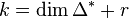 instead of
  .
.
The following example illustrates this option. We consider a complete intersection of codimension 2 in :
palp$ nef.x -S -T
Degrees and weights  `d1 w11 w12 ... d2 w21 w22 ...'
  or `#lines #colums' (= `PolyDim #Points' or `#Points PolyDim'):
4 1 1 1 1
4 1 1 1 1 M:35 4 N:5 4  codim=2 #part=2


#points in largest cone:
layer:  1 #p:        6 #ip:        0
layer:  2 #p:       21 #ip:        1
layer:  3 #p:       56 #ip:        6
layer:  4 #p:      125 #ip:       21
layer:  5 #p:      246 #ip:       56


#points in largest cone:
layer:  1 #p:       20 #ip:        0
layer:  2 #p:      105 #ip:        1
layer:  3 #p:      336 #ip:       20
layer:  4 #p:      825 #ip:      105
layer:  5 #p:     1716 #ip:      336
H:[0] P:0 V:2 3       0sec  0cpu
np=1 d:0 p:1    0sec     0cpu
One of the two nef partitions is a projection and is not analyzed. The output for the remaining nef partition has two blocks:
The first block counts the numbers of points (after #p:) and points in the relative interior (after #ip:) of the Gorenstein cone at degrees  . Hence


With these data we can compute

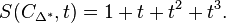
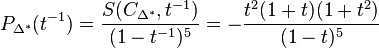
Since the Ehrhart polynomial  has degree at most , we can make the ansatz S(C_{\Delta^*},t)
 and we find from the relation
 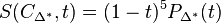 that
that
Hence
and

in agreement with the values for found above.
The same computation can be done for the dual Gorenstein cone with the data from the second block of the output.
-s
The option -s also includes nef partitions in the output which are related to symmetries of the weight matrix. Note that the option -s does not print all possible nef partitions as those corresponding to projections (cf. option -P) or direct products (cf. option -D) are left out.
Expample: Complete intersection of codimension 2 in . We add the option -Lv in order to print the vertices and the weight matrix.
palp$ nef.x -s -Lv
Degrees and weights  `d1 w11 w12 ... d2 w21 w22 ...'
  or `#lines #columns' (= `PolyDim #Points' or `#Points PolyDim'):
3 1 1 1 0 0 0 3 0 0 0 1 1 1
3 1 1 1 0 0 0  3 0 0 0 1 1 1 M:100 9 N:7 6  codim=2 #part=31
4 6 Vertices in N-lattice:
    0    0    0    1    0   -1
    0    0    1    0    0   -1
   -1    0    0    0    1    0
   -1    1    0    0    0    0
------------------------------
    1    1    0    0    1    0  d=3  codim=2
    0    0    1    1    0    1  d=3  codim=2
H:20 [24] P:2 V:4 5   (1 2) (1 2)     0sec  0cpu
H:20 [24] P:4 V:0 5   (1 2) (1 2)     0sec  0cpu
H:20 [24] P:5 V:0 4   (2 1) (0 3)     0sec  0cpu
H:20 [24] P:6 V:0 4 5   (2 1) (1 2)     0sec  0cpu
H:20 [24] P:8 V:1 5   (1 2) (1 2)     1sec  0cpu
H:20 [24] P:9 V:1 4   (2 1) (0 3)     0sec  0cpu
H:20 [24] P:10 V:1 4 5   (2 1) (1 2)     0sec  0cpu
H:20 [24] P:11 V:0 1   (2 1) (0 3)     0sec  0cpu
H:20 [24] P:12 V:0 1 5   (2 1) (1 2)     0sec  0cpu
H:20 [24] P:14 V:2 3   (0 3) (2 1)     0sec  0cpu
H:20 [24] P:16 V:2 5   (0 3) (2 1)     0sec  0cpu
H:20 [24] P:17 V:2 4   (1 2) (1 2)     0sec  0cpu
H:20 [24] P:18 V:2 4 5   (1 2) (2 1)     0sec  0cpu
H:20 [24] P:19 V:0 2   (1 2) (1 2)     0sec  0cpu
H:20 [24] P:20 V:0 2 5   (1 2) (2 1)     1sec  0cpu
H:20 [24] P:21 V:0 2 4   (2 1) (1 2)     0sec  0cpu
H:20 [24] P:22 V:1 3   (1 2) (1 2)     0sec  0cpu
H:20 [24] P:23 V:1 2   (1 2) (1 2)     0sec  0cpu
H:20 [24] P:24 V:1 2 5   (1 2) (2 1)     0sec  0cpu
H:20 [24] P:25 V:1 2 4   (2 1) (1 2)     0sec  0cpu
H:20 [24] P:26 V:0 3   (1 2) (1 2)     0sec  0cpu
H:20 [24] P:27 V:0 1 2   (2 1) (1 2)     0sec  0cpu
H:20 [24] P:28 V:3 4   (1 2) (1 2)     1sec  0cpu
H:20 [24] P:29 V:3 5   (0 3) (2 1)     0sec  0cpu
np=24 d:1 p:6    0sec     0cpu
Note that the weight matrix is symmetric under permutations of the vertices labeled by 0,1,4 and those labeled by 2,3,5. Furthermore there only exist three pairs of degrees of the complete intersection (up to exchange within a pair): {(1,2),(1,2)},{(0,3),(2,1)},{(1,2),(2,1)}. Therefore we conclude that there are only three inequivalent nef partitions. This is indeed confirmed by calling nef without the option -s:
palp$ nef.x -Lv
Degrees and weights  `d1 w11 w12 ... d2 w21 w22 ...'
  or `#lines #columns' (= `PolyDim #Points' or `#Points PolyDim'):
3 1 1 1 0 0 0 3 0 0 0 1 1 1
3 1 1 1 0 0 0  3 0 0 0 1 1 1 M:100 9 N:7 6  codim=2 #part=5
4 6 Vertices in N-lattice:
    0    0    0    1    0   -1
    0    0    1    0    0   -1
   -1    0    0    0    1    0
   -1    1    0    0    0    0
------------------------------
    1    1    0    0    1    0  d=3  codim=2
    0    0    1    1    0    1  d=3  codim=2
H:20 [24] P:1 V:3 4 5   (1 2) (2 1)     0sec  0cpu
H:20 [24] P:2 V:3 5   (0 3) (2 1)     0sec  0cpu
H:20 [24] P:3 V:4 5   (1 2) (1 2)     0sec  0cpu
np=3 d:1 p:1    0sec     0cpu
-n
The option -n prints the points of the polytope in the N-lattice only if there is at least one nef partition which does not correspond to a projection or a direct product. If there is no nef partition the polytope is not printed. In addition the number of nef partitions, the codimension and the number of points and vertices in the M- and N-lattice polytope is printed.
Example with nef partition: Codimension 2 complete intersection in
palp$ nef.x -n
Degrees and weights  `d1 w11 w12 ... d2 w21 w22 ...'
  or `#lines #columns' (= `PolyDim #Points' or `#Points PolyDim'):
4 1 1 1 1
4 1 1 1 1 M:35 4 N:5 4  codim=2 #part=2
3 5  Points of Poly in N-Lattice:
   -1    0    0    1    0
   -1    0    1    0    0
   -1    1    0    0    0
Example without a nef partition:
palp$ nef.x -n
Degrees and weights  `d1 w11 w12 ... d2 w21 w22 ...'
  or `#lines #columns' (= `PolyDim #Points' or `#Points PolyDim'):
6 3 2 1 0 0 6 3 0 0 2 1
6 3 2 1 0 0  6 3 0 0 2 1 M:21 5 N:12 5  codim=2 #part=0
Here the N-lattice polytope is not printed.
Example: no output of the polytope if there is only a nef partition corresponding to a projection:
Degrees and weights  `d1 w11 w12 ... d2 w21 w22 ...'
  or `#lines #columns' (= `PolyDim #Points' or `#Points PolyDim'):
6 3 2 1 0 0 3 1 0 0 1 1
6 3 2 1 0 0  3 1 0 0 1 1 M:24 6 N:9 5  codim=2 #part=1
We can use the option -P to check that the nef partition corresponding a projection:
palp$ nef.x -P
Degrees and weights  `d1 w11 w12 ... d2 w21 w22 ...'
  or `#lines #columns' (= `PolyDim #Points' or `#Points PolyDim'):
6 3 2 1 0 0 3 1 0 0 1 1
6 3 2 1 0 0  3 1 0 0 1 1 M:24 6 N:9 5  codim=2 #part=1
H:[0] P:0 V:4  DP      0sec  0cpu
np=0 d:0 p:1    0sec     0cpu
-v
The option -v prints the size of the matrix of vertices, the number of points and the vertices of the polytope that has been entered (M-lattice or N-lattice, depending on the input!). If the input is the weight matrix the M-lattice polytope is analyzed. The output is printed in a single line with the character E as seperator. Furthermore one can limit the output to polytopes whose number of points is limited to a lower and an upper bound:
- -v -u#, where # is an integer > 0, only gives output if the polytope has at most # points. The default value is the parameter POINT_Nmax which fixes the maximal number of points of a polytope at compilation.
- -v -l#, where # is an integer > 0, only gives output if the polytope has at least # points.The default value is 0.
After closing the program a summary is printed. It contains information on how many of the polytopes examined satisfy the bounds and how many polytopes with # of points have been found.
Example: Complete intersections of codimesnsion 2 in and with the weight matrices as input and without bounds.
palp$ nef.x -v
Degrees and weights  `d1 w11 w12 ... d2 w21 w22 ...'
  or `#lines #columns' (= `PolyDim #Points' or `#Points PolyDim'):
4 1 1 1 1
3 4 P:35 E   -1    3   -1   -1E   -1   -1    3   -1E   -1   -1   -1    3
Degrees and weights  `d1 w11 w12 ... d2 w21 w22 ...'
  or `#lines #columns' (= `PolyDim #Points' or `#Points PolyDim'):
3 1 1 1 0 0 0 3 0 0 0 1 1 1
4 9 P:100 E   -1    2   -1   -1    2   -1   -1    2   -1E   -1   -1    2   -1   -1    2   -1   -1    2E   -1   -1   -1    2    2    2   -1   -1   -1E   -1   -1   -1   -1   -1   -1    2    2    2
Degrees and weights  `d1 w11 w12 ... d2 w21 w22 ...'
  or `#lines #columns' (= `PolyDim #Points' or `#Points PolyDim'):


2  of  2

  35#    1
 100#    1
Since we have entered a weight matrix the M-lattice polytope is analyzed. Let us discuss the first line of output:
3 4 P:35 E -1 3 -1 -1E -1 -1 3 -1E -1 -1 -1 3
The first two numbers indicate the number of rows and columns of the matrix of vertices in the M-lattice polytope. P:35 indicates that the M-lattice polytope has 35 points. The vertices of the M-lattice polytope are then written in one line with the seperator E. The output of the second example is analogous. After we quit PALP by hitting enter without input the following output is given:
2  of  2

  35#    1
 100#    1
This means that 2 out of the 2 polytopes analyzed satisfy the bounds and that there is one polytope with 35 points and one with 100.
Example: Same example as above but with the upper bound for the number of points set to 50:
palp$ nef.x -v -u50
Degrees and weights  `d1 w11 w12 ... d2 w21 w22 ...'
  or `#lines #columns' (= `PolyDim #Points' or `#Points PolyDim'):
4 1 1 1 1
3 4 P:35 E   -1    3   -1   -1E   -1   -1    3   -1E   -1   -1   -1    3
Degrees and weights  `d1 w11 w12 ... d2 w21 w22 ...'
  or `#lines #columns' (= `PolyDim #Points' or `#Points PolyDim'):
3 1 1 1 0 0 0 3 0 0 0 1 1 1
Degrees and weights  `d1 w11 w12 ... d2 w21 w22 ...'
  or `#lines #columns' (= `PolyDim #Points' or `#Points PolyDim'):


1  of  2

  35#    1
Now the second polytope exceeds the upper bound for the points as it has 100 points (cf. previous example). There is no output for the second polytope and the summary indicates that only one of the two polytopes analyzed satisfies the bounds.
Example: same example as above but now we enter the N-lattice polytope and search for polytopes which have at least 7 points in the N-lattice.
Degrees and weights  `d1 w11 w12 ... d2 w21 w22 ...'
  or `#lines #columns' (= `PolyDim #Points' or `#Points PolyDim'):
3 4
Type the 12 coordinates as dim=3 lines with #pts=4 columns:
   -1    0    0    1
   -1    0    1    0
   -1    1    0    0
Degrees and weights  `d1 w11 w12 ... d2 w21 w22 ...'
  or `#lines #columns' (= `PolyDim #Points' or `#Points PolyDim'):
4 6
Type the 24 coordinates as dim=4 lines with #pts=6 columns:
    0    0    0    1    0   -1
    0    0    1    0    0   -1
   -1    0    0    0    1    0
   -1    1    0    0    0    0
4 6 P:7 E    0    0    0    1    0   -1E    0    0    1    0    0   -1E   -1    0    0    0    1    0E   -1    1    0    0    0    0
Degrees and weights  `d1 w11 w12 ... d2 w21 w22 ...'
  or `#lines #columns' (= `PolyDim #Points' or `#Points PolyDim'):


1  of  2

   7#    1
There is no output for the first polytope because it has less than 7 vertices. As one can check using option -Lp the N-lattice polytope has only 5 points. There is output for the second polytope since it has seven points and therefore satisfies the bound.
-m
The option -m returns a Minkowski sum decomposition of codimension 2  with specified degrees
  . The input data is a single weight vector which will be part of a combined weight system describing a polytope
  in the lattice , and a pair of degrees
  that add up to the degree of the weight vector. The following example taken from hep-th/0410018 illustrates this option
palp$ nef.x -m
type degrees and weights [d  w1 w2 ... wk d=d_1 d_2]: 14 1 1 1 1 4 6 d=2 12
14 1 1 1 1 4 6 d=2 12 M:1270 12 N:11 7  codim=2 #part=2
 d=12 2H:3 243 [-480] P:0 V:3 5       6sec  6cpu
np=1 d:0 p:1    0sec     0cpu
We consider the weighted projective space  specified by the weight vector 14 1 1 1 1 4 6 of degree
  . We are looking for a combined weight system describing a polytope and decomposition of into a Minkowski sum such that the degrees of the parts
  of the corresponding nef-partition are
  and
and  , respectively, with
  . The output indeed yields a polytope and such a nef-partition. To understand the output in more detail we repeat the computation with the option -Lv:
palp$ nef.x -Lv -m
type degrees and weights [d  w1 w2 ... wk d=d_1 d_2]: 14 1 1 1 1 4 6  d=2 12
14 1 1 1 1 4 6 d=2 12 M:1270 12 N:11 7  codim=2 #part=2
5 7 Vertices in N-lattice:
    0   -1    0    0    0    1    0
    0   -1    1    0    0    0    0
    0   -1    0    1    0    0    0
    0   -4    0    0    1    0   -2
    1   -6    0    0    0    0   -3
-----------------------------------
    6    1    1    1    4    1    0  d=14  codim=0
    3    0    0    0    2    0    1  d=6  codim=3
 d=12 2H:3 243 [-480] P:0 V:3 5   (2 12) (0 6)     7sec  6cpu
np=1 d:0 p:1    0sec     0cpu
Let be the standard basis of . From the columns of the subsequent 5 by 7 array of numbers, we read off that the 7 vertices are
 .
.
There are two linearly independent linear relations:
 ,
,
whose degrees are 14 and 6, respectively. The nef-partition of and its degrees are then as follows:

The Hodge numbers and the Euler number of the corresponding Calabi-Yau threefold are  . We observe that the polytope is specified by a combined weight system containing the weight vector 6 3 2 0 0 0 0 1 besides the given weight vector 14 6 4 1 1 1 1. Because of this, the Calabi-Yau 3-fold is, however, not a complete intersection of codimension 2 in the weighted projective space since the corresponding polytope only admits a nef-partition with degree (8,6) and not (2,12) as the following computation shows
palp$ nef.x -Lv
Degrees and weights  `d1 w11 w12 ... d2 w21 w22 ...'
  or `#lines #colums' (= `PolyDim #Points' or `#Points PolyDim'):
14 1 1 1 1 4 6
14 1 1 1 1 4 6 M:1271 13 N:10 8  codim=2 #part=2
5 8 Vertices in N-lattice:
    0   -1    0    0    0    1    0    0
    0   -1    1    0    0    0    0    0
    0   -1    0    1    0    0    0    0
    0   -4    0    0    1    0   -1   -1
    1   -6    0    0    0    0   -1   -2
----------------------------------------
    6    1    1    1    4    1    0    0  d=14  codim=0
    1    0    0    0    1    0    1    0  d=3  codim=3
    2    0    0    0    1    0    0    1  d=4  codim=3
H:1 149 [-296] P:1 V:3 4 5 7  8   (6 8) (1 2) (2 2)     2sec  1cpu
np=1 d:0 p:1    2sec     1cpu
-R
The option -R prints the vertices of the polytope in the N-lattice if it is not reflexive.
Example: We enter the weight matrix of a polytope which is not reflexive:
palp$ nef.x -R
Degrees and weights  `d1 w11 w12 ... d2 w21 w22 ...'
  or `#lines #columns' (= `PolyDim #Points' or `#Points PolyDim'):
6 3 2 1 0 0 5 0 0 1 1 3
3 4  Vertices of P:
   -1    1    0    0
    0    1   -1    1
   -1    0    0    0
The same output is given if we enter the N-lattice polytope itself. Without the option -R there is not output if the polytope is not reflexive:
palp$ nef.x
Degrees and weights  `d1 w11 w12 ... d2 w21 w22 ...'
  or `#lines #columns' (= `PolyDim #Points' or `#Points PolyDim'):
6 3 2 1 0 0 5 0 0 1 1 3
Degrees and weights  `d1 w11 w12 ... d2 w21 w22 ...'
  or `#lines #columns' (= `PolyDim #Points' or `#Points PolyDim'):
-V
The option -V prints the vertices of the polytope in the N-lattice together with the standard output. In contrast to the option -Lv the information about the linear relations is not given. Furthermore, in the lines containing the nef partitions the additional information about the degrees is left out. The option -V also works for non-reflexive polytopes.
Example: Complete intersection of codimension 2 in
palp$ nef.x -V
Degrees and weights  `d1 w11 w12 ... d2 w21 w22 ...'
  or `#lines #columns' (= `PolyDim #Points' or `#Points PolyDim'):
4 1 1 1 1
4 1 1 1 1 M:35 4 N:5 4  codim=2 #part=2
3 4  Vertices of P:
   -1    0    0    1
   -1    0    1    0
   -1    1    0    0
H:[0] P:0 V:2 3       0sec  0cpu
np=1 d:0 p:1    0sec     0cpu
We can also enter the M-lattice polytope to get the same result:
palp$ nef.x -V
Degrees and weights  `d1 w11 w12 ... d2 w21 w22 ...'
  or `#lines #columns' (= `PolyDim #Points' or `#Points PolyDim'):
3 4
Type the 12 coordinates as dim=3 lines with #pts=4 columns:
   -1    3   -1   -1
   -1   -1    3   -1
   -1   -1   -1    3
M:35 4 N:5 4  codim=2 #part=2
3 4  Vertices of P:
   -1    0    0    1
   -1    0    1    0
   -1    1    0    0
H:[0] P:0 V:2 3       0sec  0cpu
np=1 d:0 p:1    0sec     0cpu
Example: If the polytope is non-reflexive the output is the same as for the option -R:
palp$ nef.x -V
Degrees and weights  `d1 w11 w12 ... d2 w21 w22 ...'
  or `#lines #columns' (= `PolyDim #Points' or `#Points PolyDim'):
6 3 2 1 0 0 5 0 0 1 1 3
3 4  Vertices of P:
   -1    1    0    0
    0    1   -1    1
   -1    0    0    0
-Q
The option -Q prints the information about the nef partitions and the Hodge numbers only if the corresponding complete intersection is a direct product (cf. option -D) up to lattice quotients. If none of the nef partitions is a direct product only the numbers of points and vertices in the M- and N-lattice, together with the codimension and the number of nef partitions is given.
Example: Complete intersection of codimension 2 in . As one can check using the option -D one of the nef partitions corresponds to a direct product:
palp$ nef.x -Q
Degrees and weights  `d1 w11 w12 ... d2 w21 w22 ...'
  or `#lines #columns' (= `PolyDim #Points' or `#Points PolyDim'):
3 1 1 1 0 0 0 3 0 0 0 1 1 1
3 1 1 1 0 0 0  3 0 0 0 1 1 1 M:100 9 N:7 6  codim=2 #part=5
H:4 [0] h1=2 P:0 V:2 3 5   D     0sec  0cpu
np=4 d:1 p:0    0sec     0cpu
Example: Complete intersection of codimension 2 in . This example has no nef partition corresponding to a direct product. Then the output looks as follows:
palp$ nef.x -Q
Degrees and weights  `d1 w11 w12 ... d2 w21 w22 ...'
  or `#lines #columns' (= `PolyDim #Points' or `#Points PolyDim'):
4 1 1 1 1
4 1 1 1 1 M:35 4 N:5 4  codim=2 #part=2
np=2 d:0 p:0    0sec     0cpu
Example: Complete intersection of codimension 2 in quotiented by  :
:
palp$ nef.x -Q
Degrees and weights  `d1 w11 w12 ... d2 w21 w22 ...'
  or `#lines #columns' (= `PolyDim #Points' or `#Points PolyDim'):
3 1 1 1 0 0 0 3 0 0 0 1 1 1/Z3: 0 1 2 0 0 0/Z3: 0 0 0 1 2 0
3 1 1 1 0 0 0  3 0 0 0 1 1 1 /Z3: 0 1 2 0 0 0 /Z3: 0 0 0 1 2 0 M:16 9 N:19 6  codim=2 #part=1
H:4 [0] h1=2 P:0 V:2 3 5  7 9 10 11 15 16   D     0sec  0cpu
np=0 d:1 p:0    0sec     0cpu
Note that the nef partition now contains more points due to the lattice refinement induced by the quotient.
???: The comment "up to lattice quotient" in the help screens may indicate that the scope of this option is larger than described here.
-g*
The option -gm returns the Gorenstein cone supported on the input polytope with the apex in the origin of the lattice , where is the codimension of the nef-partition, specified by the option -c*. The integer m takes either of the three values 0, 1, or 2. The default value for m is 1.
The standard output is changed as follows: The lines containing the information about the nef-partition including the Hodge numbers, the parts of the nef-partition etc. are suppressed. Instead, for each nef-partition the points of the Gorenstein cone are printed in the following form:
D n Points of PG: (nv=#)
    #    #      ...      #    #

    .    .      ...      .    .
    .    .      ...      .    .
    .    .      ...      .    .

    #    #      ...      #    #
The interpretation depends on the integer m:
- If m = 0 then the first line says that the points of the -dimensional polytope supporting the Gorenstein cone in the lattice
 are given by the subsequent lines with entries. The number # in nv=# denotes the number of vertices of the polytope. The means that the polytope is given by points which are the columns of the subsequent array of numbers #. This is similar to the option -Lp except that the linear relations are not displayed. The order of the points is first the vertices, then the non-vertex points with the origin at the end.
- If m = 2 then the first line says that the points of the
 -dimensional Gorenstein cone
  in the lattice with -dimensional support polytope are given by the subsequent lines with entries. The number # in nv=# denotes the number of vertices of the polytope. The means that the Gorenstein cone is given by points which are the columns of the subsequent
  array of numbers #. Recall that a partition
  of the set of vertices
  of into disjoint subsets
 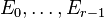 is called a nef-partition if there exist integral upper convex piecewise linear support functions
  such that
  if
if  and
and  otherwise. Each column of this array of numbers therefore takes the form
 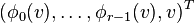 . The points are ordered in the same way as for m=0. Note that since the origin
  belongs to every part of the nef-partition, it appears times, each time another of the support functions being equal to 1.
- If m = 1 then the output is the same as for m=2 except that the redundant r-th direction of the Gorenstein cone is suppressed since it can be determined from the other r-1 directions depending on whether there are r-1 zeros or not.
Note that in all the cases an arbitrary basis of will be chosen.
This option -g2 is very useful in the context of the combinatorial mirror symmetry of nef-partitions of reflexive lattice polytopes by Batyrev and Borisov, see arXiv:alg-geom/9310001, arXiv:alg-geom/9412017, and arXiv:math/0703456v2. For more details see the option -d*. The option -g2 automatically sets the flag -p.
The following examples illustrate this option. We consider complete intersections of codimension 2 in discussed in arXiv:0704.0449[hep-th ]. We choose the enter the polytope by its points in the lattice in order to keep them in the given order. Hence we have to use the option -N.
palp$ nef.x -g0
Degrees and weights  `d1 w11 w12 ... d2 w21 w22 ...'
  or `#lines #colums' (= `PolyDim #Points' or `#Points PolyDim'):
3 1 1 1 0 0 0 0 0  2 0 0 0 1 1 0 0 0  3 0 0 0 0 0 1 1 1
3 1 1 1 0 0 0 0 0  2 0 0 0 1 1 0 0 0  3 0 0 0 0 0 1 1 1 M:300 18 N:9 8  codim=2 #part=15
5 9 Points of PG: (nv=8)
    0    0    0    0    1    0   -1    0    0
    0    0    1    0    0    0   -1    0    0
    0    0    0    1    0    0    0   -1    0
   -1    0    0    0    0    1    0    0    0
   -1    1    0    0    0    0    0    0    0
5 9 Points of PG: (nv=8)
    0    0    0    0    1    0   -1    0    0
    0    0    1    0    0    0   -1    0    0
    0    0    0    1    0    0    0   -1    0
   -1    0    0    0    0    1    0    0    0
   -1    1    0    0    0    0    0    0    0
5 9 Points of PG: (nv=8)
    0    0    0    0    1    0   -1    0    0
    0    0    1    0    0    0   -1    0    0
    0    0    0    1    0    0    0   -1    0
   -1    0    0    0    0    1    0    0    0
   -1    1    0    0    0    0    0    0    0
5 9 Points of PG: (nv=8)
    0    0    0    0    1    0   -1    0    0
    0    0    1    0    0    0   -1    0    0
    0    0    0    1    0    0    0   -1    0
   -1    0    0    0    0    1    0    0    0
   -1    1    0    0    0    0    0    0    0
5 9 Points of PG: (nv=8)
    0    0    0    0    1    0   -1    0    0
    0    0    1    0    0    0   -1    0    0
    0    0    0    1    0    0    0   -1    0
   -1    0    0    0    0    1    0    0    0
   -1    1    0    0    0    0    0    0    0
5 9 Points of PG: (nv=8)
    0    0    0    0    1    0   -1    0    0
    0    0    1    0    0    0   -1    0    0
    0    0    0    1    0    0    0   -1    0
   -1    0    0    0    0    1    0    0    0
   -1    1    0    0    0    0    0    0    0
5 9 Points of PG: (nv=8)
    0    0    0    0    1    0   -1    0    0
    0    0    1    0    0    0   -1    0    0
    0    0    0    1    0    0    0   -1    0
   -1    0    0    0    0    1    0    0    0
   -1    1    0    0    0    0    0    0    0
5 9 Points of PG: (nv=8)
    0    0    0    0    1    0   -1    0    0
    0    0    1    0    0    0   -1    0    0
    0    0    0    1    0    0    0   -1    0
   -1    0    0    0    0    1    0    0    0
   -1    1    0    0    0    0    0    0    0
5 9 Points of PG: (nv=8)
    0    0    0    0    1    0   -1    0    0
    0    0    1    0    0    0   -1    0    0
    0    0    0    1    0    0    0   -1    0
   -1    0    0    0    0    1    0    0    0
   -1    1    0    0    0    0    0    0    0
5 9 Points of PG: (nv=8)
    0    0    0    0    1    0   -1    0    0
    0    0    1    0    0    0   -1    0    0
    0    0    0    1    0    0    0   -1    0
   -1    0    0    0    0    1    0    0    0
   -1    1    0    0    0    0    0    0    0
5 9 Points of PG: (nv=8)
    0    0    0    0    1    0   -1    0    0
    0    0    1    0    0    0   -1    0    0
    0    0    0    1    0    0    0   -1    0
   -1    0    0    0    0    1    0    0    0
   -1    1    0    0    0    0    0    0    0
The nef-partitions for this example were discussed in the illustrating example for the standard output. For each of the 11 nef-partitions the 9 points of the 5-dimensional polytope are displayed, there are 8 vertices and the origin. Since they only differ by their nef-partitions which are suppressed by the choice of m=0, they are all the same. Compare this to the output of the option -Lp.
palp$ nef.x -N -Lp
Degrees and weights  `d1 w11 w12 ... d2 w21 w22 ...'
  or `#lines #colums' (= `PolyDim #Points' or `#Points PolyDim'):
5 8
Type the 40 coordinates as dim=5 lines with #pts=8 colums:
 1  0 -1  0  0  0  0  0
 0  1 -1  0  0  0  0  0
 0  0  0  1 -1  0  0  0
 0  0  0  0  0  1  0 -1
 0  0  0  0  0  0  1 -1
M:300 18 N:9 8  codim=2 #part=15
5 9  Points of Poly in N-Lattice:
    1    0   -1    0    0    0    0    0    0
    0    1   -1    0    0    0    0    0    0
    0    0    0    1   -1    0    0    0    0
    0    0    0    0    0    1    0   -1    0
    0    0    0    0    0    0    1   -1    0
---------------------------------------------
    1    1    1    0    0    0    0    0  d=3  codim=3
    0    0    0    1    1    0    0    0  d=2  codim=4
    0    0    0    0    0    1    1    1  d=3  codim=3
H:3 51 [-96] P:0 V:2 3 4 7   (1 2) (2 0) (1 2)     1sec  0cpu
H:3 51 [-96] P:1 V:2 4 6 7   (1 2) (1 1) (2 1)     1sec  1cpu
H:3 60 [-114] P:2 V:2 4 7   (1 2) (1 1) (1 2)     2sec  1cpu
H:3 51 [-96] P:3 V:2 6 7   (1 2) (0 2) (2 1)     1sec  0cpu
H:3 69 [-132] P:4 V:2 7   (1 2) (0 2) (1 2)     1sec  0cpu
H:9 27 [-36] P:5 V:3 4 6 7   (0 3) (2 0) (2 1)     0sec  0cpu
H:3 75 [-144] P:6 V:3 4 7   (0 3) (2 0) (1 2)     1sec  0cpu
H:19 19 [0] P:8 V:4 5 6 7   (0 3) (1 1) (3 0)     0sec  0cpu
H:6 51 [-90] P:9 V:4 6 7   (0 3) (1 1) (2 1)     1sec  0cpu
H:3 75 [-144] P:10 V:4 7   (0 3) (1 1) (1 2)     1sec  0cpu
H:3 75 [-144] P:13 V:6 7   (0 3) (0 2) (2 1)     0sec  0cpu
np=11 d:2 p:2    0sec     0cpu
With the choice of m=2 we obtain the information about the partition in terms of the Gorenstein cone. Let be the standard basis of . Let denote the vertices of the polytope in the lattice with

Consider the nef-partition P:8 above that was the focus of arXiv:0704.0449[hep-th ].

With -g2 we get
palp$ nef.x -N -g2
Degrees and weights  `d1 w11 w12 ... d2 w21 w22 ...'
  or `#lines #colums' (= `PolyDim #Points' or `#Points PolyDim'):
5 8
Type the 40 coordinates as dim=5 lines with #pts=8 colums:
 1  0 -1  0  0  0  0  0
 0  1 -1  0  0  0  0  0
 0  0  0  1 -1  0  0  0
 0  0  0  0  0  1  0 -1
 0  0  0  0  0  0  1 -1
M:300 18 N:9 8  codim=2 #part=15
7 10 Points of PG: (nv=8)
    1    1    0    0    0    1    1    0    0    1
    0    0    1    1    1    0    0    1    1    0
    1    0   -1    0    0    0    0    0    0    0
    0    1   -1    0    0    0    0    0    0    0
    0    0    0    1   -1    0    0    0    0    0
    0    0    0    0    0    1    0   -1    0    0
    0    0    0    0    0    0    1   -1    0    0
7 10 Points of PG: (nv=8)
    1    1    0    1    0    1    0    0    0    1
    0    0    1    0    1    0    1    1    1    0
    1    0   -1    0    0    0    0    0    0    0
    0    1   -1    0    0    0    0    0    0    0
    0    0    0    1   -1    0    0    0    0    0
    0    0    0    0    0    1    0   -1    0    0
    0    0    0    0    0    0    1   -1    0    0
7 10 Points of PG: (nv=8)
    1    1    0    1    0    1    1    0    0    1
    0    0    1    0    1    0    0    1    1    0
    1    0   -1    0    0    0    0    0    0    0
    0    1   -1    0    0    0    0    0    0    0
    0    0    0    1   -1    0    0    0    0    0
    0    0    0    0    0    1    0   -1    0    0
    0    0    0    0    0    0    1   -1    0    0
7 10 Points of PG: (nv=8)
    1    1    0    1    1    1    0    0    0    1
    0    0    1    0    0    0    1    1    1    0
    1    0   -1    0    0    0    0    0    0    0
    0    1   -1    0    0    0    0    0    0    0
    0    0    0    1   -1    0    0    0    0    0
    0    0    0    0    0    1    0   -1    0    0
    0    0    0    0    0    0    1   -1    0    0
7 10 Points of PG: (nv=8)
    1    1    0    1    1    1    1    0    0    1
    0    0    1    0    0    0    0    1    1    0
    1    0   -1    0    0    0    0    0    0    0
    0    1   -1    0    0    0    0    0    0    0
    0    0    0    1   -1    0    0    0    0    0
    0    0    0    0    0    1    0   -1    0    0
    0    0    0    0    0    0    1   -1    0    0
7 10 Points of PG: (nv=8)
    1    1    1    0    0    1    0    0    0    1
    0    0    0    1    1    0    1    1    1    0
    1    0   -1    0    0    0    0    0    0    0
    0    1   -1    0    0    0    0    0    0    0
    0    0    0    1   -1    0    0    0    0    0
    0    0    0    0    0    1    0   -1    0    0
    0    0    0    0    0    0    1   -1    0    0
7 10 Points of PG: (nv=8)
    1    1    1    0    0    1    1    0    0    1
    0    0    0    1    1    0    0    1    1    0
    1    0   -1    0    0    0    0    0    0    0
    0    1   -1    0    0    0    0    0    0    0
    0    0    0    1   -1    0    0    0    0    0
    0    0    0    0    0    1    0   -1    0    0
    0    0    0    0    0    0    1   -1    0    0
7 10 Points of PG: (nv=8)
    1    1    1    1    0    0    0    0    0    1
    0    0    0    0    1    1    1    1    1    0
    1    0   -1    0    0    0    0    0    0    0
    0    1   -1    0    0    0    0    0    0    0
    0    0    0    1   -1    0    0    0    0    0
    0    0    0    0    0    1    0   -1    0    0
    0    0    0    0    0    0    1   -1    0    0
7 10 Points of PG: (nv=8)
    1    1    1    1    0    1    0    0    0    1
    0    0    0    0    1    0    1    1    1    0
    1    0   -1    0    0    0    0    0    0    0
    0    1   -1    0    0    0    0    0    0    0
    0    0    0    1   -1    0    0    0    0    0
    0    0    0    0    0    1    0   -1    0    0
    0    0    0    0    0    0    1   -1    0    0
7 10 Points of PG: (nv=8)
    1    1    1    1    0    1    1    0    0    1
    0    0    0    0    1    0    0    1    1    0
    1    0   -1    0    0    0    0    0    0    0
    0    1   -1    0    0    0    0    0    0    0
    0    0    0    1   -1    0    0    0    0    0
    0    0    0    0    0    1    0   -1    0    0
    0    0    0    0    0    0    1   -1    0    0
7 10 Points of PG: (nv=8)
    1    1    1    1    1    1    0    0    0    1
    0    0    0    0    0    0    1    1    1    0
    1    0   -1    0    0    0    0    0    0    0
    0    1   -1    0    0    0    0    0    0    0
    0    0    0    1   -1    0    0    0    0    0
    0    0    0    0    0    1    0   -1    0    0
    0    0    0    0    0    0    1   -1    0    0
The 7 x 10 array of points corresponding to the nef-partition P:8 is the 8th in the list (since P:7 is not displayed, cf. the standard output)
7 10 Points of PG: (nv=8)
    1    1    1    1    0    0    0    0    0    1
    0    0    0    0    1    1    1    1    1    0
    1    0   -1    0    0    0    0    0    0    0
    0    1   -1    0    0    0    0    0    0    0
    0    0    0    1   -1    0    0    0    0    0
    0    0    0    0    0    1    0   -1    0    0
    0    0    0    0    0    0    1   -1    0    0
Since the first four vertices  and
and  are in , we have
  and
and  , hence the corresponding points of the Gorenstein cone take the form
  for
for  . The next four vertices
  and
and  are in
  , we have
  and
and  , hence the corresponding points of the Gorenstein cone take the form
  for
for  . Finally, the origin always belongs to every part of the nef-partition, hence it appears as often as the codimension which here is
  . So
. So  and
and  . Once with
  and
and  and once with
  and
and  .
.
-d*
The option -dm returns the dual Gorenstein cone supported on the polytope with the apex in the origin of the lattice , where is the codimension of the nef-partition, specified by the option -c*. The integer m takes either of the three values 0, 1, or 2. The integer m takes either of the three values 0, 1, or 2. The default value for m is 1. The option -d2 automatically sets the flag -p.
The polytope is related to the input polytope via combinatorial mirror symmetry, and is not its dual unless  . In particular, this option can be used to determine the polytope for each of the nef-partitions of the given polytope . The polytope can then be further analyzed with poly.x.
The combinatorial mirror symmetry of nef-partitions of reflexive lattice polytopes by Batyrev and Borisov, see arXiv:alg-geom/9310001, arXiv:alg-geom/9412017, and arXiv:math/0703456v2, can be summarized in the following diagram:
The polytopes  , and are all in
  , hence they appear on the left-hand side below . On the right-hand side below
  , the polytopes
  , and are all in
  . The angle brackets denote the convex hull, and the plus signs denote the Minkowski sum.
The relation in the middle  expresses the polytopes
  in terms of the
  and vice versa, for
  , the parentheses denoting the scalar product between and . If a nef-partition of the polytope is given, then the polytopes are obtained as the convex hull
Polar duality relates  to , and to . Mirror symmetry relates to , and to .
The following examples illustrate this option. We consider complete intersections of codimension 2 in discussed in arXiv:0704.0449[hep-th ]. We choose the enter the polytope by its points in the lattice in order to keep them in the given order. Hence we have to use the option -N. The nef-partitions for this example were discussed in the illustrating example for the standard output and for the option -g*.
palp$ nef.x -N -d2 Degrees and weights `d1 w11 w12 ... d2 w21 w22 ...' or `#lines #colums' (= `PolyDim #Points' or `#Points PolyDim'): 5 8 Type the 40 coordinates as dim=5 lines with #pts=8 colums: 1 0 -1 0 0 0 0 0 0 1 -1 0 0 0 0 0 0 0 0 1 -1 0 0 0 0 0 0 0 0 1 0 -1 0 0 0 0 0 0 1 -1 M:300 18 N:9 8 codim=2 #part=15 7 63 Points of dual PG: (nv=27) 1 0 1 0 0 1 1 1 0 0 0 0 0 1 1 0 0 0 0 0 1 0 0 0 0 1 0 1 1 1 1 1 1 1 1 1 1 0 1 0 0 0 0 1 1 1 1 1 1 0 0 0 1 1 1 1 1 1 1 1 1 0 1 0 1 0 1 1 0 0 0 1 1 1 1 1 0 0 1 1 1 1 1 0 1 1 1 1 0 1 0 0 0 0 0 0 0 0 0 0 1 0 1 1 1 1 0 0 0 0 0 0 1 1 1 0 0 0 0 0 0 0 0 0 1 0 -1 0 1 1 0 -1 -1 -1 0 0 0 1 1 1 1 1 1 0 0 0 -1 0 0 0 0 -1 1 0 0 0 0 0 0 0 0 0 0 0 0 0 0 0 0 -1 1 -1 1 1 -1 1 1 1 -1 -1 -1 -1 -1 -1 -1 -1 -1 0 0 -1 1 -1 0 1 1 1 -1 1 1 0 0 0 -1 -1 0 0 1 1 0 -1 0 0 0 0 1 0 -1 -1 -1 -1 -1 -1 0 0 0 0 0 0 0 1 1 1 0 -1 1 -1 -1 -1 0 0 0 1 -1 -1 1 0 0 0 0 0 0 0 0 1 0 1 -1 0 0 0 1 1 1 -1 -1 0 0 1 1 -1 -1 -1 0 1 1 -1 -1 0 -1 0 0 0 0 0 0 0 0 0 0 0 0 0 0 0 0 0 0 0 0 0 0 0 0 0 0 0 0 0 0 0 0 0 0 0 0 -1 0 -1 0 0 1 -1 -1 1 0 0 1 0 1 -1 1 0 1 0 0 1 1 0 1 0 -1 0 -1 -1 -1 0 0 1 -1 -1 -1 0 0 1 1 0 0 1 1 -1 0 0 0 0 0 0 1 -1 -1 0 0 0 -1 -1 0 -1 0 0 -1 1 1 1 1 -1 -1 1 0 0 1 0 0 -1 -1 0 0 0 0 1 -1 0 0 0 0 1 1 -1 0 1 -1 0 -1 -1 0 1 -1 1 -1 0 0 1 0 -1 0 0 -1 0 0 0 1 0 0 0 -1 -1 0 1 0 -1 -1 0 0 7 72 Points of dual PG: (nv=36) 0 0 0 1 0 0 0 1 0 1 1 0 0 0 0 0 1 1 0 0 0 0 0 1 1 1 1 1 0 1 1 1 1 1 1 1 1 0 0 1 0 1 1 1 0 1 0 0 1 1 1 1 0 1 0 0 0 1 0 1 0 0 1 1 0 1 0 0 1 0 0 1 1 1 1 0 1 1 1 0 1 0 0 1 1 1 1 1 0 0 1 1 1 1 1 0 0 0 0 0 1 0 0 0 0 0 0 0 0 1 1 0 1 0 0 0 1 0 1 1 0 0 0 0 1 0 1 1 1 0 1 0 1 1 0 0 1 0 1 1 0 1 1 0 0 0 1 -1 0 0 0 -1 0 1 1 1 1 1 1 1 -1 -1 0 0 0 0 0 -1 -1 -1 -1 -1 0 1 -1 -1 -1 1 1 1 -1 0 0 -1 0 0 -1 0 1 0 1 1 0 -1 0 0 0 0 0 0 0 0 0 -1 0 0 0 0 1 0 1 1 -1 0 0 0 0 1 0 1 1 1 1 -1 0 -1 -1 0 0 0 0 0 1 1 1 1 0 0 0 -1 -1 -1 -1 -1 0 -1 1 1 1 -1 -1 -1 0 1 1 0 1 -1 0 0 0 0 0 0 0 0 0 -1 0 0 0 0 0 -1 1 0 1 1 -1 -1 0 -1 0 0 0 0 0 0 0 1 1 0 0 1 1 0 1 -1 -1 0 0 0 1 1 -1 -1 0 0 0 1 1 -1 0 0 -1 -1 0 0 -1 0 0 -1 0 0 -1 0 0 0 0 0 0 0 0 -1 0 0 -1 -1 0 0 1 -1 1 1 0 -1 1 0 1 1 -1 0 1 -1 1 1 -1 0 0 0 0 0 0 -1 0 2 0 -1 0 0 -1 2 0 0 2 0 0 -1 2 0 0 2 0 -1 0 -1 0 -1 2 -1 -1 0 -1 -1 0 -1 0 1 1 -1 0 -1 -1 -1 0 -1 1 1 0 -1 -1 0 0 -1 1 1 1 -1 0 0 1 1 -1 -1 0 0 1 1 -1 1 0 0 -1 1 1 1 1 -1 -1 1 1 0 0 -1 -1 1 -1 -1 0 0 -1 -1 1 -1 -1 1 0 0 0 0 -1 1 1 0 0 1 0 0 0 -1 0 0 0 0 1 1 0 1 -1 0 0 1 0 0 0 0 -1 0 0 1 0 0 -1 0 0 1 0 0 -1 0 0 -1 0 0 7 90 Points of dual PG: (nv=35) 1 0 1 0 1 1 1 0 0 0 0 1 1 1 1 1 1 0 1 0 1 0 1 0 0 0 0 1 1 1 1 0 0 0 0 0 1 1 1 1 1 1 1 1 1 1 1 1 1 1 1 1 1 1 1 1 1 1 1 1 1 1 1 1 1 1 1 1 1 1 1 1 1 1 1 1 1 1 1 1 1 1 1 1 1 1 1 1 1 1 0 1 0 1 0 0 0 1 1 1 1 0 0 0 0 0 0 1 0 1 0 1 0 1 1 1 1 0 0 0 0 1 1 1 1 1 0 0 0 0 0 0 0 0 0 0 0 0 0 0 0 0 0 0 0 0 0 0 0 0 0 0 0 0 0 0 0 0 0 0 0 0 0 0 0 0 0 0 0 0 0 0 0 0 0 0 0 0 0 0 -1 0 1 1 -1 -1 -1 0 0 0 1 1 1 -1 1 -1 -1 0 -1 0 -1 0 -1 1 0 1 0 1 1 -1 -1 0 0 0 1 1 -1 -1 -1 -1 -1 -1 0 -1 0 -1 -1 -1 0 0 0 0 0 0 0 0 0 0 0 0 1 -1 -1 0 0 1 -1 1 1 0 1 0 0 -1 -1 -1 -1 0 -1 -1 -1 1 -1 0 0 -1 -1 0 -1 0 -1 1 -1 0 -1 1 1 1 0 0 0 -1 -1 1 -1 -1 -1 0 -1 1 1 1 1 0 0 0 0 -1 -1 -1 1 0 1 1 0 0 0 0 0 0 0 0 0 1 0 1 1 1 -1 -1 -1 -1 -1 -1 0 0 0 0 0 0 -1 0 -1 0 -1 -1 1 -1 -1 -1 -1 -1 -1 0 0 -1 -1 -1 -1 0 -1 -1 1 0 -1 -1 0 0 0 0 -1 1 0 1 0 0 0 0 1 1 0 0 0 -1 -1 0 0 0 -1 0 -1 0 -1 0 0 0 0 -1 -1 -1 0 1 1 1 1 1 0 0 0 0 0 0 -1 0 -1 0 0 -1 0 0 0 0 0 0 0 0 0 0 -1 0 -1 -1 -1 -1 -1 0 -1 0 0 -1 -1 -1 -1 -1 -1 -1 -1 -1 0 -1 0 -1 -1 -1 -1 0 -1 -1 -1 0 -1 0 -1 0 -1 1 -1 0 1 0 0 1 -1 -1 -1 1 -1 0 -1 1 1 0 -1 1 1 0 0 1 -1 1 -1 0 1 0 1 0 -1 -1 -1 0 0 1 1 -1 -1 0 0 0 -1 -1 -1 0 0 1 -1 -1 -1 0 -1 1 0 -1 0 0 0 -1 -1 0 0 -1 0 -1 1 0 -1 -1 0 -1 -1 0 0 -1 0 -1 0 0 -1 0 1 0 -1 1 1 1 1 -1 -1 1 0 0 1 -1 -1 1 1 -1 -1 1 1 0 -1 0 -1 0 0 0 0 -1 -1 -1 1 1 0 0 0 0 -1 0 1 -1 0 -1 -1 0 0 -1 0 0 -1 0 1 -1 0 -1 -1 0 1 -1 1 -1 -1 0 0 0 -1 0 0 -1 0 1 0 0 -1 -1 1 0 -1 -1 0 0 -1 0 -1 -1 0 0 -1 -1 -1 0 7 72 Points of dual PG: (nv=27) 0 0 0 1 1 0 0 1 1 0 1 1 1 1 0 0 1 1 1 1 0 1 1 1 1 1 1 1 1 1 1 0 0 1 1 0 1 0 0 1 1 1 1 1 0 1 0 0 1 1 1 1 1 1 1 1 1 1 1 1 1 1 1 1 1 1 1 1 1 1 0 1 1 1 1 0 0 1 1 0 0 1 0 0 0 0 1 1 0 0 0 0 1 0 0 0 0 0 0 0 0 0 0 1 1 0 0 1 0 1 1 0 0 0 0 0 1 0 1 1 0 0 0 0 0 0 0 0 0 0 0 0 0 0 0 0 0 0 0 0 0 0 1 0 0 0 1 -1 -1 0 0 -1 -1 0 1 1 1 1 1 1 -1 -1 -1 -1 0 -1 -1 -1 -1 1 1 0 0 -1 0 0 0 -1 0 0 -1 0 0 0 1 1 1 -1 1 -1 1 1 -1 -1 0 -1 -1 -1 -1 -1 -1 -1 -1 0 0 0 0 0 0 0 0 0 0 0 0 0 0 1 0 1 1 1 1 -1 -1 0 -1 -1 -1 -1 0 0 1 1 1 1 0 -1 -1 -1 -1 -1 -1 0 0 0 0 0 0 0 -1 1 0 1 1 -1 -1 -1 -1 -1 0 0 0 0 0 1 -1 1 0 0 0 0 -1 1 -1 -1 -1 -1 -1 0 0 0 -1 -1 0 0 0 0 0 0 0 1 -1 0 0 1 -1 0 1 1 -1 -1 0 0 1 1 -1 -1 0 1 1 -1 -1 1 -1 0 0 0 -1 0 0 0 -1 0 -1 0 0 -1 0 0 0 0 0 0 0 0 -1 0 -1 0 -1 1 1 1 0 0 0 0 1 1 1 1 1 1 0 0 -1 -1 0 0 0 0 0 -1 -1 2 0 -1 -1 0 0 -1 0 -1 2 0 0 -1 0 -1 2 0 -1 0 -1 -1 -1 -1 -1 -1 -1 1 1 0 -1 0 0 1 1 -1 -1 -1 0 -1 0 -1 1 1 -1 -1 0 -1 -1 -1 -1 0 0 0 -1 -1 -1 -1 0 -1 -1 0 0 -1 0 -1 0 0 -1 1 1 1 1 -1 -1 1 1 1 0 0 0 0 -1 -1 0 0 0 0 -1 0 0 0 0 1 1 0 1 1 1 -1 0 0 1 0 0 -1 0 0 0 1 0 0 0 0 -1 0 0 1 0 0 1 0 1 0 0 0 1 0 0 1 0 0 1 0 0 1 0 0 0 0 7 117 Points of dual PG: (nv=26) 1 0 1 0 1 1 1 1 0 0 1 1 1 1 1 1 1 1 1 1 1 1 0 0 0 0 0 1 1 1 1 1 1 1 1 1 1 1 1 1 1 1 1 1 1 1 1 1 1 1 1 1 1 1 1 1 1 1 1 1 1 1 1 1 1 1 1 1 1 1 1 1 1 1 1 1 1 1 1 1 1 1 1 1 1 1 1 1 1 1 1 1 1 1 1 1 1 1 1 1 1 1 1 1 1 1 1 1 1 1 1 1 1 1 1 1 1 0 1 0 1 0 0 0 0 1 1 0 0 0 0 0 0 0 0 0 0 0 0 1 1 1 1 1 0 0 0 0 0 0 0 0 0 0 0 0 0 0 0 0 0 0 0 0 0 0 0 0 0 0 0 0 0 0 0 0 0 0 0 0 0 0 0 0 0 0 0 0 0 0 0 0 0 0 0 0 0 0 0 0 0 0 0 0 0 0 0 0 0 0 0 0 0 0 0 0 0 0 0 0 0 0 0 0 0 0 0 0 0 0 0 0 0 0 -1 0 1 1 -1 -1 -1 -1 0 0 -1 -1 -1 1 1 1 1 1 -1 -1 -1 -1 0 0 0 1 1 0 -1 -1 0 -1 -1 -1 -1 -1 -1 -1 -1 -1 -1 -1 -1 -1 -1 -1 -1 -1 -1 0 0 0 0 0 0 0 0 0 0 0 0 -1 0 0 1 1 1 1 1 1 1 1 -1 1 -1 -1 0 -1 -1 0 -1 -1 -1 -1 -1 -1 -1 -1 -1 0 -1 -1 -1 -1 -1 0 0 0 0 0 0 0 0 0 0 0 0 0 1 0 1 1 0 -1 0 -1 0 -1 1 -1 0 -1 1 1 1 0 0 -1 1 1 -1 -1 -1 -1 -1 -1 -1 -1 1 0 1 1 0 0 0 0 0 0 -1 -1 -1 -1 -1 -1 0 0 0 0 0 0 1 1 1 1 1 1 -1 -1 -1 -1 -1 -1 0 0 0 0 0 0 -1 -1 0 -1 -1 -1 -1 -1 -1 -1 -1 1 -1 0 -1 -1 -1 -1 0 0 0 0 0 0 0 0 1 1 0 1 1 1 -1 -1 -1 -1 -1 -1 -1 -1 0 0 0 0 0 0 -1 -1 -1 -1 -1 -1 0 -1 0 0 -1 0 1 0 1 1 1 -1 0 0 -1 -1 -1 1 1 -1 -1 -1 1 1 -1 1 0 0 0 0 0 -1 -1 -1 -1 0 0 0 0 0 0 0 0 0 0 0 0 0 0 0 0 0 0 0 0 0 0 0 0 0 0 0 0 -1 0 -1 -1 -1 -1 0 0 0 0 0 0 -1 -1 -1 -1 1 -1 1 1 -1 -1 1 1 1 1 1 1 -1 1 -1 1 1 -1 -1 -1 1 1 1 1 1 1 1 1 1 1 1 1 -1 1 -1 1 1 -1 -1 -1 -1 0 -1 0 -1 0 -1 1 -1 -1 1 0 -1 1 -1 1 -1 -1 1 -1 1 -1 1 -1 0 1 0 1 0 -1 1 -1 0 -1 -1 -1 0 0 1 -1 -1 -1 0 0 1 -1 -1 -1 0 0 1 -1 -1 -1 0 0 1 -1 -1 -1 0 -1 1 0 1 0 -1 -1 -1 -1 0 0 1 0 -1 0 0 -1 -1 0 0 -1 -1 -1 -1 -1 0 0 1 0 -1 1 0 0 0 -1 0 -1 -1 -1 0 0 1 -1 -1 -1 0 0 1 0 -1 -1 0 0 0 -1 -1 0 0 -1 1 1 1 1 -1 -1 1 0 0 1 -1 -1 -1 -1 1 -1 -1 -1 -1 -1 1 1 0 0 0 0 -1 -1 0 0 -1 0 1 -1 0 -1 -1 0 1 -1 0 -1 -1 0 1 -1 0 -1 -1 0 1 -1 0 -1 -1 0 1 -1 0 -1 0 -1 -1 0 -1 0 1 -1 0 -1 0 0 -1 -1 0 0 -1 0 1 1 -1 0 1 -1 0 -1 0 0 -1 -1 0 -1 0 -1 -1 0 1 -1 0 -1 -1 0 1 -1 0 -1 0 0 1 -1 0 -1 -1 -1 0 0 7 48 Points of dual PG: (nv=15) 0 0 1 1 1 0 0 0 0 1 1 1 1 1 1 1 1 1 1 1 1 1 1 0 0 0 0 0 1 1 1 1 1 1 1 1 1 1 0 1 0 0 0 0 0 1 0 1 1 1 0 0 0 1 1 1 1 0 0 0 0 0 0 0 0 0 0 0 0 0 0 1 1 1 1 1 0 0 0 0 0 0 0 0 0 0 1 0 1 1 1 1 1 0 1 0 0 0 -1 2 -1 0 0 0 0 -1 -1 2 2 -1 -1 -1 -1 -1 0 0 0 0 0 0 0 0 0 0 0 0 0 1 1 1 1 1 1 -1 0 -1 0 0 0 0 0 -1 0 0 0 0 2 -1 -1 0 0 0 0 2 2 -1 -1 -1 -1 0 1 0 -1 -1 -1 0 0 0 0 0 0 0 1 1 1 -1 -1 -1 0 0 0 1 0 0 0 0 0 0 0 1 0 0 -1 1 0 0 0 1 -1 1 -1 0 0 0 0 0 0 0 0 0 0 0 0 0 0 0 0 0 0 0 0 0 0 0 0 0 0 0 0 0 -1 0 -1 1 -1 1 1 0 0 0 0 0 -1 -1 -1 2 0 0 2 0 -1 0 -1 0 -1 -1 0 -1 -1 -1 0 -1 -1 0 0 1 1 2 -1 -1 0 -1 -1 0 -1 -1 0 -1 1 0 1 0 0 1 1 -1 0 0 -1 1 1 1 1 -1 1 -1 -1 0 0 0 0 0 0 1 0 0 0 1 0 0 1 -1 1 -1 0 -1 0 1 0 0 1 0 0 1 0 0 -1 0 0 0 0 -1 0 1 0 0 7 69 Points of dual PG: (nv=15) 1 0 1 1 0 1 1 1 1 1 1 0 0 0 0 1 1 1 1 1 1 1 1 1 1 1 1 1 1 1 1 1 1 1 1 1 1 0 1 0 1 1 1 1 1 1 1 1 1 1 1 1 1 1 1 1 1 1 1 1 1 1 1 1 1 1 1 0 1 0 1 0 0 1 0 0 0 0 0 0 1 1 1 1 0 0 0 0 0 0 0 0 0 0 0 0 0 0 0 0 0 0 0 0 0 0 1 0 1 0 0 0 0 0 0 0 0 0 0 0 0 0 0 0 0 0 0 0 0 0 0 0 0 0 0 0 1 0 -1 0 2 -1 0 -1 -1 -1 2 2 -1 0 0 0 0 -1 -1 -1 -1 -1 -1 -1 -1 -1 -1 -1 -1 0 0 0 0 0 0 0 0 0 0 0 0 0 0 0 0 0 0 0 1 1 1 1 1 1 1 1 1 1 1 1 -1 2 -1 2 2 -1 -1 -1 -1 0 0 -1 0 -1 2 0 2 -1 2 -1 -1 -1 0 0 0 0 1 1 1 1 1 1 -1 2 0 2 2 -1 -1 -1 -1 -1 -1 -1 0 0 0 0 0 0 0 1 1 1 1 1 1 -1 -1 -1 -1 -1 -1 0 0 0 0 0 0 0 -1 0 -1 -1 0 0 -1 0 0 0 0 1 0 0 -1 0 0 0 0 0 0 1 1 -1 -1 0 0 0 0 0 0 0 0 0 0 0 0 0 0 0 0 0 0 0 0 0 0 0 0 0 0 0 0 0 0 0 0 0 0 0 0 0 0 0 0 0 0 0 0 0 0 0 0 0 0 0 0 0 0 -1 0 -1 -1 0 1 -1 -1 1 -1 1 1 0 1 0 -1 -1 -1 0 0 1 0 -1 1 0 0 0 -1 -1 -1 0 0 1 -1 -1 -1 0 0 1 1 -1 -1 -1 0 0 1 -1 -1 -1 0 0 1 -1 -1 -1 0 0 1 -1 -1 0 0 0 -1 0 -1 -1 0 0 -1 1 1 1 1 -1 1 -1 -1 -1 -1 0 0 0 0 -1 0 1 -1 0 -1 0 0 -1 -1 0 -1 -1 0 1 -1 0 -1 -1 0 1 -1 1 -1 0 -1 0 1 -1 0 -1 -1 0 1 -1 0 -1 -1 0 1 -1 0 -1 -1 0 0 -1 0 0 -1 0 1 0 0 7 40 Points of dual PG: (nv=12) 0 0 1 1 1 0 0 0 1 1 1 0 1 1 1 1 0 0 1 0 0 0 0 1 1 1 1 1 1 0 0 1 0 0 0 0 0 1 0 1 1 1 0 0 0 1 1 1 0 0 0 1 0 0 0 0 1 1 0 1 1 1 1 0 0 0 0 0 0 1 1 0 1 1 1 1 1 0 1 0 0 0 -1 2 -1 0 0 0 -1 2 -1 0 -1 1 0 -1 0 0 1 0 0 0 0 -1 0 1 1 -1 0 0 0 0 0 0 0 0 0 0 0 0 0 0 2 -1 -1 0 0 0 2 -1 -1 0 1 0 -1 1 0 0 -1 0 0 0 0 0 1 -1 0 0 1 0 0 -1 0 0 0 0 0 0 0 0 0 1 0 0 0 1 1 0 -1 -1 -1 0 0 -1 0 -1 0 0 -1 0 0 0 0 0 0 0 0 -1 -1 1 1 -1 1 1 1 1 1 -1 0 0 -1 -1 0 0 0 2 -1 -1 0 0 0 2 0 0 0 0 -1 -1 0 0 0 1 1 0 0 0 0 0 0 -1 -1 0 0 0 0 1 1 0 0 0 -1 2 0 0 0 -1 -1 2 0 0 0 -1 0 0 0 0 0 1 0 -1 1 -1 0 0 0 0 0 0 0 0 1 0 -1 0 1 -1 0 0 0 0 7 72 Points of dual PG: (nv=24) 0 0 1 1 1 0 0 0 1 1 1 1 1 1 1 1 1 0 1 1 1 1 1 1 1 1 1 1 1 1 1 1 1 1 1 1 1 1 1 1 1 1 1 1 1 1 0 0 1 1 1 1 1 1 1 1 1 1 1 1 1 1 1 1 0 1 0 0 1 1 0 1 1 1 0 0 0 1 1 1 0 0 0 0 0 0 0 0 0 1 0 0 0 0 0 0 0 0 0 0 0 0 0 0 0 0 0 0 0 0 0 0 0 0 0 0 0 0 1 1 0 0 0 0 0 0 0 0 0 0 0 0 0 0 0 0 1 0 1 1 0 0 1 0 0 0 -1 2 -1 0 0 0 -1 -1 -1 2 2 2 -1 -1 -1 0 -1 2 -1 -1 2 -1 0 -1 0 0 0 1 -1 -1 -1 -1 -1 -1 0 -1 1 0 0 0 0 0 -1 0 0 0 1 0 0 0 1 1 1 1 1 1 0 1 1 -1 1 -1 0 -1 0 0 0 0 0 0 0 0 2 -1 -1 0 0 0 2 2 2 -1 -1 -1 -1 -1 -1 0 2 -1 -1 2 -1 -1 0 0 0 1 -1 -1 0 0 0 1 1 1 -1 1 0 -1 -1 -1 0 0 1 -1 0 0 -1 1 1 1 -1 -1 -1 0 0 0 0 -1 0 0 0 0 0 1 0 0 1 1 0 0 0 1 0 0 0 1 0 1 -1 -1 0 -1 -1 0 -1 -1 0 0 -1 -1 -1 0 0 0 -1 -1 -1 -1 -1 -1 0 0 0 0 0 0 -1 -1 -1 0 0 0 0 0 -1 -1 0 0 -1 0 0 0 0 0 0 0 0 0 -1 -1 -1 -1 -1 -1 1 -1 1 1 -1 -1 0 0 0 0 -1 -1 -1 2 0 0 0 -1 -1 0 -1 -1 0 -1 -1 2 -1 -1 -1 0 0 0 -1 -1 -1 0 -1 0 -1 -1 0 -1 -1 0 0 0 -1 -1 -1 0 -1 -1 -1 -1 1 1 -1 -1 -1 0 -1 -1 0 -1 -1 0 0 -1 0 -1 -1 0 0 -1 1 1 -1 -1 0 0 -1 1 1 1 1 -1 1 -1 0 1 0 0 1 0 0 1 0 -1 0 0 0 0 0 0 1 0 0 0 1 0 0 1 0 0 1 0 0 0 1 0 1 0 0 1 0 0 -1 0 0 0 1 0 0 1 0 0 1 0 0 1 0 1 0 0 0 1 -1 0 0 1 0 0 7 126 Points of dual PG: (nv=23) 1 0 1 1 1 1 1 0 1 1 1 1 0 0 1 1 1 0 1 0 1 1 1 1 1 1 1 1 1 1 1 1 1 1 1 1 1 1 1 1 1 1 1 1 1 1 1 1 1 1 1 1 1 1 1 1 1 1 1 1 1 1 1 1 1 1 1 1 1 1 1 1 1 1 1 1 1 1 1 1 1 1 1 1 1 1 1 1 1 1 1 1 1 1 1 1 1 1 1 1 1 1 1 1 1 1 1 1 1 1 1 1 1 1 1 1 1 1 1 1 1 1 1 1 1 1 0 1 0 0 0 0 0 1 0 0 0 0 1 1 0 0 0 1 0 1 0 0 0 0 0 0 0 0 0 0 0 0 0 0 0 0 0 0 0 0 0 0 0 0 0 0 0 0 0 0 0 0 0 0 0 0 0 0 0 0 0 0 0 0 0 0 0 0 0 0 0 0 0 0 0 0 0 0 0 0 0 0 0 0 0 0 0 0 0 0 0 0 0 0 0 0 0 0 0 0 0 0 0 0 0 0 0 0 0 0 0 0 0 0 0 0 0 0 0 0 0 0 0 0 0 0 -1 0 2 -1 -1 -1 -1 0 2 2 -1 -1 0 0 -1 2 -1 0 -1 0 -1 2 2 -1 0 0 0 0 0 0 0 0 0 0 1 1 1 1 1 1 1 1 1 1 1 1 -1 2 -1 -1 2 2 0 0 -1 -1 -1 -1 -1 0 -1 -1 -1 -1 -1 -1 -1 -1 -1 -1 -1 -1 -1 -1 -1 -1 -1 -1 0 0 0 0 0 0 0 0 0 0 -1 0 0 0 0 0 0 0 0 1 1 1 1 1 1 1 1 1 1 1 1 -1 2 0 2 2 -1 -1 -1 -1 -1 -1 0 -1 -1 0 0 0 -1 0 -1 2 -1 2 2 0 -1 -1 -1 -1 0 0 2 -1 -1 0 2 0 2 -1 -1 -1 0 0 0 0 1 1 1 1 1 1 -1 -1 -1 -1 -1 -1 0 0 0 0 0 0 0 -1 0 0 -1 -1 -1 0 -1 -1 1 -1 -1 -1 0 0 0 0 0 0 1 1 1 1 1 1 1 2 1 2 2 1 -1 -1 -1 -1 -1 -1 0 0 0 0 1 0 -1 1 1 1 1 1 1 -1 -1 -1 -1 -1 -1 0 0 0 0 0 0 2 -1 0 -1 -1 1 0 0 -1 -1 2 -1 2 0 -1 -1 0 -1 1 0 0 0 0 0 0 0 0 0 0 1 1 -1 -1 -1 0 -1 0 -1 -1 -1 -1 -1 -1 -1 -1 -1 -1 -1 -1 -1 -1 -1 -1 -1 -1 -1 -1 -1 -1 -1 -1 -1 -1 -1 -1 -1 -1 -1 -1 -1 -1 -1 0 -1 0 0 -1 0 0 0 0 0 0 0 0 0 0 0 0 -1 0 -1 0 0 -1 0 0 0 0 0 0 0 0 0 0 -1 0 -1 0 0 0 0 0 0 0 0 0 0 0 0 0 0 0 0 0 0 -1 0 -1 0 0 -1 -1 -1 -1 -1 -1 -1 -1 -1 -1 -1 0 -1 0 -1 -1 -1 1 -1 0 1 -1 1 -1 1 0 -1 -1 -1 1 1 0 -1 1 -1 1 -1 0 0 1 -1 -1 -1 0 0 1 -1 -1 -1 0 0 1 -1 -1 -1 0 0 1 1 -1 0 -1 0 0 1 -1 0 -1 -1 0 0 -1 -1 -1 -1 0 0 1 -1 -1 -1 0 0 1 0 -1 -1 0 0 -1 -1 -1 -1 0 0 1 -1 -1 -1 0 0 1 -1 -1 -1 -1 0 0 1 -1 -1 -1 0 0 1 -1 -1 -1 0 0 1 -1 -1 -1 0 0 1 0 -1 -1 0 0 0 0 -1 -1 0 0 -1 1 1 1 1 -1 -1 1 -1 -1 -1 -1 0 0 1 1 1 0 -1 0 -1 -1 -1 -1 1 -1 0 -1 -1 0 1 -1 0 -1 -1 0 1 -1 0 -1 -1 0 1 -1 0 -1 -1 0 0 0 -1 0 -1 0 0 0 0 -1 0 1 -1 0 1 -1 0 -1 -1 0 1 -1 0 -1 -1 0 -1 -1 0 1 -1 0 1 -1 0 -1 -1 0 1 -1 0 -1 0 -1 0 1 -1 0 -1 -1 0 1 -1 0 -1 -1 0 1 -1 0 -1 0 0 -1 -1 0 -1 -1 1 0 -1 0 0 -1 -1 -1 -1 0 7 96 Points of dual PG: (nv=21) 0 0 1 1 1 0 1 1 1 1 1 1 1 1 1 1 1 1 1 1 1 1 1 1 1 1 1 1 1 1 1 1 1 1 1 1 1 1 1 1 1 1 1 1 1 1 0 0 1 1 1 1 1 1 1 1 1 1 1 1 1 1 1 1 1 1 1 1 1 1 1 1 1 1 1 1 1 1 1 1 1 1 1 1 1 1 1 1 1 1 1 1 1 1 0 1 1 1 0 0 0 1 0 0 0 0 0 0 0 0 0 0 0 0 0 0 0 0 0 0 0 0 0 0 0 0 0 0 0 0 0 0 0 0 0 0 0 0 0 0 0 0 1 1 0 0 0 0 0 0 0 0 0 0 0 0 0 0 0 0 0 0 0 0 0 0 0 0 0 0 0 0 0 0 0 0 0 0 0 0 0 0 0 0 0 0 0 0 0 0 1 0 0 0 -1 2 -1 0 -1 2 -1 -1 -1 2 2 -1 -1 -1 2 -1 -1 2 -1 1 1 1 -1 -1 0 -1 -1 -1 -1 -1 -1 -1 -1 -1 -1 -1 -1 0 0 0 0 0 -1 -1 0 0 1 0 0 0 1 1 1 1 1 1 2 2 2 1 0 0 -1 -1 -1 -1 -1 -1 -1 0 -1 1 0 0 0 0 0 0 0 0 0 0 1 1 1 1 1 1 0 0 0 0 0 0 0 0 2 -1 2 0 -1 -1 -1 2 2 -1 -1 2 2 -1 -1 -1 -1 -1 -1 0 0 -1 0 0 1 -1 -1 -1 0 0 0 1 1 1 2 2 2 -1 -1 -1 0 0 1 1 0 0 -1 1 1 1 -1 -1 -1 0 0 0 -1 -1 -1 -1 0 1 0 0 0 0 1 1 1 -1 1 0 -1 -1 -1 -1 0 0 0 1 1 1 -1 -1 -1 0 0 0 0 1 -1 0 0 0 0 0 1 1 -1 0 1 -1 -1 1 1 1 1 -1 -1 1 -1 -1 1 -1 -1 -1 -1 -1 -1 -1 -1 0 0 0 0 0 0 0 0 0 0 0 0 0 0 0 0 0 -1 -1 0 0 -1 0 0 0 0 0 0 0 0 0 0 0 0 -1 -1 -1 -1 1 1 1 1 1 1 -1 -1 -1 -1 1 1 1 1 1 1 1 1 1 1 1 1 1 1 1 -1 -1 -1 -1 0 0 0 0 -1 -1 -1 2 -1 -1 -1 0 -1 0 -1 0 -1 0 0 0 -1 -1 -1 -1 0 0 0 -1 0 -1 -1 0 -1 -1 0 -1 -1 0 -1 -1 0 -1 -1 0 -1 -1 -1 -1 1 1 -1 -1 -1 0 -1 -1 0 -1 -1 0 -1 -1 0 -1 0 -1 -1 -1 -1 0 -1 -1 0 0 0 -1 -1 -1 -1 0 -1 -1 0 -1 -1 0 -1 -1 0 -1 -1 0 -1 -1 -1 -1 0 0 -1 1 1 1 1 -1 1 1 1 0 0 0 0 0 0 0 0 0 0 0 0 1 0 0 0 0 0 0 1 0 0 1 0 0 1 0 0 1 0 0 1 0 0 1 0 1 -1 0 0 0 1 0 0 1 0 0 1 0 0 1 0 1 0 1 1 0 1 0 0 1 0 0 0 0 1 0 1 0 0 1 0 0 1 0 0 1 0 0 1 0 1 0 0 0 0 0
For each of the 11 nef-partitions of the input polytope (which all had the same points) we get a 7-dimensional dual Gorenstein cone supported on a 5-dimensional polytope. For each nef-partition the number of points and the number of vertices differ in general. The nef-partition of interest in in arXiv:0704.0449[hep-th ] and in the description of the option -g* was P:8, i.e. the 8th in the list above:
7 40 Points of dual PG: (nv=12)
   0   0   1   1   1   0   0   0   1   1   1   0   1   1   1   1   0   0   1   0   0   0   0   1   1   1   1   1   1   0   0   1   0   0   0   0   0   1   0   1
   1   1   0   0   0   1   1   1   0   0   0   1   0   0   0   0   1   1   0   1   1   1   1   0   0   0   0   0   0   1   1   0   1   1   1   1   1   0   1   0
   0   0  -1   2  -1   0   0   0  -1   2  -1   0  -1   1   0  -1   0   0   1   0   0   0   0  -1   0   1   1  -1   0   0   0   0   0   0   0   0   0   0   0   0
   0   0   2  -1  -1   0   0   0   2  -1  -1   0   1   0  -1   1   0   0  -1   0   0   0   0   0   1  -1   0   0   1   0   0  -1   0   0   0   0   0   0   0   0
   0   1   0   0   0   1   1   0  -1  -1  -1   0   0  -1   0  -1   0   0  -1   0   0   0   0   0   0   0   0  -1  -1   1   1  -1   1   1   1   1   1  -1   0   0
  -1  -1   0   0   0   2  -1  -1   0   0   0   2   0   0   0   0  -1  -1   0   0   0   1   1   0   0   0   0   0   0  -1  -1   0   0   0   0   1   1   0   0   0
  -1   2   0   0   0  -1  -1   2   0   0   0  -1   0   0   0   0   0   1   0  -1   1  -1   0   0   0   0   0   0   0   0   1   0  -1   0   1  -1   0   0   0   0
We see that the polytope has 39 points (note that the interior point appears times) and 12 vertices. Let be the standard basis of . Let  denote the vertices of the polytope with


From the first two rows of the above output we can read off the nef partition  of :
of :

We can check this by feeding the vertices back into nef.x with the options -N and -Lv:
palp$ nef.x -N -Lv
Degrees and weights  `d1 w11 w12 ... d2 w21 w22 ...'
  or `#lines #colums' (= `PolyDim #Points' or `#Points PolyDim'):
5 12
Type the 60 coordinates as dim=5 lines with #pts=12 colums:
   0   0  -1   2  -1   0   0   0  -1   2  -1   0
   0   0   2  -1  -1   0   0   0   2  -1  -1   0
   0   1   0   0   0   1   1   0  -1  -1  -1   0
  -1  -1   0   0   0   2  -1  -1   0   0   0   2
  -1   2   0   0   0  -1  -1   2   0   0   0  -1
M:24 15 N:39 12  codim=2 #part=2
5 12 Vertices in N-lattice:
    0    0   -1    2   -1    0    0    0   -1    2   -1    0
    0    0    2   -1   -1    0    0    0    2   -1   -1    0
    0    1    0    0    0    1    1    0   -1   -1   -1    0
   -1   -1    0    0    0    2   -1   -1    0    0    0    2
   -1    2    0    0    0   -1   -1    2    0    0    0   -1
------------------------------------------------------------
    1    1    2    2    0    1    0    0    0    0    2    0  d=9  codim=0
    1    1    1    1    0    0    0    0    0    0    1    1  d=6  codim=0
    1    1    2    0    2    1    0    0    0    2    0    0  d=9  codim=0
    1    1    1    0    1    0    0    0    0    1    0    1  d=6  codim=0
    1    1    1    0    0    1    0    0    0    1    1    0  d=6  codim=0
    2    2    1    0    0    0    0    0    0    1    1    2  d=9  codim=0
    1    1    0    2    2    1    0    0    2    0    0    0  d=9  codim=0
    1    1    0    1    1    0    0    0    1    0    0    1  d=6  codim=0
    1    1    0    1    0    1    0    0    1    0    1    0  d=6  codim=0
    2    2    0    1    0    0    0    0    1    0    1    2  d=9  codim=0
    1    1    0    0    1    1    0    0    1    1    0    0  d=6  codim=0
    2    2    0    0    1    0    0    0    1    1    0    2  d=9  codim=0
    3    3    0    0    0    3    0    0    2    2    2    0  d=15  codim=0
    3    3    0    0    0    0    0    0    1    1    1    3  d=12  codim=0
    1    0    1    1    0    1    0    1    0    0    1    0  d=6  codim=0
    1    0    1    0    1    1    0    1    0    1    0    0  d=6  codim=0
    2    0    1    0    0    2    0    2    0    1    1    0  d=9  codim=0
    1    0    0    1    1    1    0    1    1    0    0    0  d=6  codim=0
    2    0    0    1    0    2    0    2    1    0    1    0  d=9  codim=0
    2    0    0    0    1    2    0    2    1    1    0    0  d=9  codim=0
    3    0    0    0    0    3    0    3    1    1    1    0  d=12  codim=0
    1    0    0    0    0    0    0    1    0    0    0    1  d=3  codim=3
    0    1    3    3    0    1    1    0    0    0    3    0  d=12  codim=0
    0    1    2    2    0    0    1    0    0    0    2    1  d=9  codim=0
    0    1    3    0    3    1    1    0    0    3    0    0  d=12  codim=0
    0    1    2    0    2    0    1    0    0    2    0    1  d=9  codim=0
    0    2    3    0    0    2    2    0    0    3    3    0  d=15  codim=0
    0    1    1    0    0    0    1    0    0    1    1    1  d=6  codim=0
    0    1    0    3    3    1    1    0    3    0    0    0  d=12  codim=0
    0    1    0    2    2    0    1    0    2    0    0    1  d=9  codim=0
    0    2    0    3    0    2    2    0    3    0    3    0  d=15  codim=0
    0    1    0    1    0    0    1    0    1    0    1    1  d=6  codim=0
    0    2    0    0    3    2    2    0    3    3    0    0  d=15  codim=0
    0    1    0    0    1    0    1    0    1    1    0    1  d=6  codim=0
    0    1    0    0    0    1    1    0    1    1    1    0  d=6  codim=0
    0    3    0    0    0    0    3    0    2    2    2    3  d=15  codim=0
    0    0    1    1    1    0    0    0    0    0    0    0  d=3  codim=3
    0    0    2    2    0    1    1    1    0    0    2    0  d=9  codim=0
    0    0    1    1    0    0    1    1    0    0    1    1  d=6  codim=0
    0    0    2    0    2    1    1    1    0    2    0    0  d=9  codim=0
    0    0    1    0    1    0    1    1    0    1    0    1  d=6  codim=0
    0    0    1    0    0    1    1    1    0    1    1    0  d=6  codim=0
    0    0    1    0    0    0    2    2    0    1    1    2  d=9  codim=0
    0    0    0    2    2    1    1    1    2    0    0    0  d=9  codim=0
    0    0    0    1    1    0    1    1    1    0    0    1  d=6  codim=0
    0    0    0    1    0    1    1    1    1    0    1    0  d=6  codim=0
    0    0    0    1    0    0    2    2    1    0    1    2  d=9  codim=0
    0    0    0    0    1    1    1    1    1    1    0    0  d=6  codim=0
    0    0    0    0    1    0    2    2    1    1    0    2  d=9  codim=0
    0    0    0    0    0    3    3    3    2    2    2    0  d=15  codim=0
    0    0    0    0    0    0    3    3    1    1    1    3  d=12  codim=0
H:19 19 [0] P:0 V:1 2 3 4 5 6  13 15 17 19 21 23 25 26 28 30 32 34 36   (6 3) (3 3) (6 3) (3 3) (3 3) (3 6) (6 3) (3 3) (3 3) (3 6) (3 3) (3 6) (6 9) (3 9) (3 3) (3 3) (3 6) (3 3) (3 6) (3 6) (3 9) (0 3) (9 3) (6 3) (9 3) (6 3) (9 6) (3 3) (9 3) (6 3) (9 6) (3 3) (9 6) (3 3) (3 3) (6 9) (3 0) (6 3) (3 3) (6 3) (3 3) (3 3) (3 6) (6 3) (3 3) (3 3) (3 6) (3 3) (3 6) (6 9) (3 9)     1sec  0cpu
H:19 19 [0] P:1 V:2 3 4 8 9 10  16 17 18 19 20 21 24 29 30 31 32 33 34   (6 3) (3 3) (6 3) (3 3) (3 3) (3 6) (6 3) (3 3) (3 3) (3 6) (3 3) (3 6) (6 9) (3 9) (3 3) (3 3) (3 6) (3 3) (3 6) (3 6) (3 9) (0 3) (9 3) (6 3) (9 3) (6 3) (9 6) (3 3) (9 3) (6 3) (9 6) (3 3) (9 6) (3 3) (3 3) (6 9) (3 0) (6 3) (3 3) (6 3) (3 3) (3 3) (3 6) (6 3) (3 3) (3 3) (3 6) (3 3) (3 6) (6 9) (3 9)     0sec  0cpu
np=2 d:0 p:0    0sec     0cpu
We see that the nef-partition P:1 agrees with . This is the starting point for further analysis of the polytopes and its polar dual .
-e
In Polynf.c there exists a procedure Einstein_Metric. It is called by the option -e of "nef.x". In order for this procedure to deal with general reflexive polytopes, one has to change the flag SMOOTH at the beginning of Polynf.c to (0). Einstein_Metric checks several symmetry properties of a reflexive polytope related to the set of roots of the associated toric variety. These are of interest with respect to the existence of Einstein-Kaehler metrics. Here, a root is a lattice point in the interior of a facet of the reflexive polytope (in the M-lattice). Centrally-symmetric roots are called semisimple. If all roots are semisimple, then ssroot=1. Only in this case PALP proceeds to check and display the following conditions: if the barycenter is 0 (bary=1), the sum of lattice points is 0 (#Psum=1), the sum of lattice points in each multiple is 0 (#kPsum=1), the group of lattice automorphisms has only the origin as a fixpoint (#symm=1). These conditions can be found explained in Chapter 5 (in particular, sections 5.5 and 5.6) of the dissertation of Benjamin Nill: http://tobias-lib.uni-tuebingen.de/dbt/volltexte/2005/1888/
Strategy for future versions
Should we keep both help screens, or try to get everything into 'nef.x -h'?
It would be good to have a documentation of the header file Nef.h: just type whatever information you can supply into the following listing, in the standard ('/* ... */') C comment format.
#define Nef_Max 	500000
#define NP_Max          500000
#define W_Nmax (POLY_Dmax+1)
#define MAXSTRING	100

#undef	WRITE_CWS
#define	WRITE_CWS

#define Pos_Max   (POLY_Dmax + 2)
#define FIB_Nmax        10*EQUA_Nmax
#define FIB_POINT_Nmax  VERT_Nmax

typedef struct {
  Long W[FIB_Nmax][FIB_POINT_Nmax];
  Long VM[FIB_POINT_Nmax][POLY_Dmax];
  int nw;
  int nv;
  int d;
  int Wmax;
} LInfo;

struct Poset_Element {
  int num, dim;
};

struct Interval {
  int min, max;
};

typedef struct Interval Interval;

typedef struct {
  struct Interval *L;
  int n;
} Interval_List;

typedef struct Poset_Element Poset_Element;

typedef struct {
  struct Poset_Element x, y;
} Poset;

typedef struct {
  struct Poset_Element *L;
  int n;
} Poset_Element_List;

typedef struct {
  int nface[Pos_Max];
  int dim;
  INCI edge[Pos_Max][FACE_Nmax];
} Cone;

typedef struct {
  Long S[2*Pos_Max];
} SPoly;

typedef struct {
  Long B[Pos_Max][Pos_Max];
} BPoly;

typedef struct {
  int E[4*(Pos_Max)][4*(Pos_Max)];
} EPoly;

typedef struct {
    Long x[POINT_Nmax][W_Nmax];
    int N, np;
} AmbiPointList;

typedef struct {
  int n;
  int nv;
  int codim;
  int S[Nef_Max][VERT_Nmax];
  int DirProduct[Nef_Max];
  int Proj[Nef_Max];
  int DProj[Nef_Max];
} PartList;

typedef struct {
  int n;
  int nv;
  int S[Nef_Max][VERT_Nmax];
} Part;

typedef struct {
  int n, y, w, p, t, S, Lv, Lp, N, u, d, g, VP, B, T, H, dd, gd,
	noconvex, Msum, Sym, V, Rv, Test, Sort, Dir, Proj, f;
} Flags;

typedef struct {
	int noconvex, Sym, Test, Sort;
} NEF_Flags;

struct Vector {
  Long x[POLY_Dmax];
};

typedef struct Vector Vector ;

typedef struct {
  struct Vector *L;
  int n;
  Long np, NP_max;						} DYN_PPL;

void part_nef(PolyPointList *, VertexNumList *, EqList *, PartList *,
	      int *, NEF_Flags *);

void Make_E_Poly(FILE *, CWS *, PolyPointList *, VertexNumList *, EqList *,
		 int *, Flags *, int *);

void Mink_WPCICY(AmbiPointList * _AP_1, AmbiPointList * _AP_2,
		 AmbiPointList * _AP);

int  IsDigit(char);

int  IntSqrt(int q);

void Die(char *);

void Print_CWS_Zinfo(CWS *);