Documentation on nef.x

nef.x is the application designed to address the following problems.

...

The corresponding routines are listed in the header file Nef.h.

Standard output

The standard output slightly depends on whether the polytope is input as a combined weight system or by a list of points. If the polytope was input as a list of points, the first line of the output takes the following form:

M:# # N:# # codim=# #part=#

Note that by default the input polytope is in the lattice M, while the output polytope is its dual in the lattice N. To change the lattice of the input polytope see the option -N. If the input was a combined weight system, the line starts with the combined weight system repeated before the symbol M.

# M:# # N:# # codim=# #part=#

where # is the sequence of numbers describing the combined weight system. Note that the combined weight system describes the output polytope in the lattice N.

The two numbers # after M correspond to the number of points and vertices of the input polytope in the lattice M, respectively.

The two numbers # after N correspond to the number of points and vertices of the output polytope in the lattice N, respectively.

The number # in codim=# is the codimension of the nef-partition. The default is 2, otherwise it is specified by the option -c*.

The number # in #part=# is the number n of all the nef-partitions that nef.x has found, up to symmetries of the underlying lattice. It specifies the number of lines that follow the first output line. If the symmetries of the underlying lattice should not be taken into account, use the option -s.

The next lines contain the information about the various nef-partitions. If the codimension is 2 they take the following form:

H:# [#] P:# V:#  #      #sec #cpu

The numbers # after H: are the Hodge numbers $h^{1,i}(X), i=1,\dots,d-1$ , where $d\,$ is the dimension of the Calabi-Yau manifold $X\,$ that can be obtained from this nef-partition.

The number # in the square brackets [#] is the Euler number of $X\,$ . Under the assumption that $h^{0,i}(X)=0, i=1,\dots,d-1$ , the remaining Hodge numbers can be computed from the ones given after H: and the Euler number. If this assumption is not satified, the Calabi-Yau manifold contains $T^2\,$ factors and the Hodge numbers $h^{0,i}(X)\,$ are nonvanishing. See the option -D for this case. In any case, the full Hodge diamond is displayed with the option -H.

The number # after P: is a counter specfiying the nef-partition. It runs from 0 to n - 1, where n is the number of nef-partitions. Note that nef-partitions corresponding to direct products and projections to nef-partitions of lower codimensions are omitted by default. To display them use the options -D and -P, respectively.

The sequence of numbers # separated by a single space after V: corresponds to the vertices that belong to the first part of the nef-partition. Note that the vertices are counted starting from 0. These numbers only make sense if the options -Lv or -Lp are used. The vertices that belong to the second part of the nef-partition are not displayed, since they are simply the remaining ones. If the polytope entered also has points that are not vertices, then the second sequence of numbers # that is separated from the first sequence by two spaces corresponds to the non-vertex points that belong to the first partition. Again, the non-vertex points that belong to the second part of the nef-partition are not displayed. For other representations of the nef-partition in terms of the Gorenstein cone see the option -g*.

The number # before sec indicates the time that was needed to compute this partition.

The number # before cpu indicates the number of CPU seconds that were needed to compute the Hodge numbers. For determining the nef-partitions without computing the Hodge numbers see the option -p.

If the codimension r is bigger than 2 the lines containing the information about the various nef-partitions take the following form:

H:# [#] P:# V0:#  # V1:#  # ... V(r-2):#  #      #sec #cpu

Now, there are r - 1 expressions of the form Vi:# #, where i runs from 0 to r - 2. Each expression consists of two sequences of numbers # separated by two spaces from each other. The first sequence of numbers # separated by a single space corresponds to the vertices that belong to the i-th part of the nef-partition. The second sequence of numbers # separated by a single space corresponds to the non-vertex points that belong to the i-th part of the nef-partition. The second sequence of numbers # is omitted if the polytope has no points that are not vertices or if the option -Lv is used.

The final line always takes the following form

np=# d:# p:#    #sec     #cpu

The number # in np=# is the number of nef-partitions which are neither direct products nor projections.

The number # after d: is the number of nef-partitions that are direct products.

The number # after p: is the number of nef-partitions that are projections. The total of the three numbers adds up to the total number of nef-partitions as indicated in the first line after #part=.

The number # before sec indicates the time that was needed to compute all the partitions.

The number # before cpu indicates the number of CPU seconds that were needed to compute the Hodge numbers of all the nef-partitions.

The following examples illustrate the standard output of nef.x. We consider complete intersections of codimension 2 in $\mathbb{P}^2\times\mathbb{P}^1\times\mathbb{P}^2$ discussed in arXiv:0704.0449. First, we enter the polytope by giving the combined weight system (which is essentially the same as a linearly independent set of linear relations) of this product of projective spaces

palp$ nef.x 
Degrees and weights  `d1 w11 w12 ... d2 w21 w22 ...'
  or `#lines #colums' (= `PolyDim #Points' or `#Points PolyDim'):
3 1 1 1 0 0 0 0 0  2 0 0 0 1 1 0 0 0  3 0 0 0 0 0 1 1 1
3 1 1 1 0 0 0 0 0  2 0 0 0 1 1 0 0 0  3 0 0 0 0 0 1 1 1 M:300 18 N:9 8  codim=2 #part=15
H:19 19 [0] P:0 V:2 4 6 7       1sec  0cpu
H:9 27 [-36] P:2 V:3 4 6 7       1sec  0cpu
H:3 51 [-96] P:3 V:3 5 6 7       1sec  1cpu
H:3 75 [-144] P:4 V:3 6 7       1sec  0cpu
H:3 51 [-96] P:6 V:4 5 6 7       2sec  1cpu
H:3 51 [-96] P:7 V:4 5 6       1sec  1cpu
H:6 51 [-90] P:8 V:4 6 7       1sec  1cpu
H:3 75 [-144] P:9 V:4 6       1sec  1cpu
H:3 60 [-114] P:10 V:5 6 7       2sec  1cpu
H:3 69 [-132] P:11 V:5 6       1sec  1cpu
H:3 75 [-144] P:12 V:6 7       1sec  0cpu
np=11 d:2 p:2    0sec     0cpu

Equivalently, we can use the option -N and enter the points of the polytope of the normal fan of $\mathbb{P}^2\times\mathbb{P}^1\times\mathbb{P}^2$

esche$ nef.x -N
Degrees and weights  `d1 w11 w12 ... d2 w21 w22 ...'
  or `#lines #colums' (= `PolyDim #Points' or `#Points PolyDim'):
5 8
Type the 40 coordinates as dim=5 lines with #pts=8 colums:
 1  0 -1  0  0  0  0  0
 0  1 -1  0  0  0  0  0
 0  0  0  1 -1  0  0  0
 0  0  0  0  0  1  0 -1
 0  0  0  0  0  0  1 -1
M:300 18 N:9 8  codim=2 #part=15
H:3 51 [-96] P:0 V:2 3 4 7       1sec  1cpu
H:3 51 [-96] P:1 V:2 4 6 7       2sec  1cpu
H:3 60 [-114] P:2 V:2 4 7       2sec  1cpu
H:3 51 [-96] P:3 V:2 6 7       1sec  1cpu
H:3 69 [-132] P:4 V:2 7       1sec  1cpu
H:9 27 [-36] P:5 V:3 4 6 7       1sec  0cpu
H:3 75 [-144] P:6 V:3 4 7       0sec  0cpu
H:19 19 [0] P:8 V:4 5 6 7       1sec  0cpu
H:6 51 [-90] P:9 V:4 6 7       1sec  1cpu
H:3 75 [-144] P:10 V:4 7       1sec  0cpu
H:3 75 [-144] P:13 V:6 7       1sec  1cpu
np=11 d:2 p:2    0sec     0cpu

Note that the nef-partitions are given in different orders. The first lines of the outputs respectively read

3 1 1 1 0 0 0 0 0  2 0 0 0 1 1 0 0 0  3 0 0 0 0 0 1 1 1 M:300 18 N:9 8  codim=2 #part=15

and

M:300 18 N:9 8  codim=2 #part=15

Hence the polytope in the lattice N has 9 points, 8 vertices and the interior point, while the polytope in the lattice M has 300 points, 18 of which are vertices. The codimension is 2 and there are 15 nef-partitions. These are listed as follows:

H:3 51 [-96] P:0 V:2 3 4 7       1sec  1cpu
H:3 51 [-96] P:1 V:2 4 6 7       2sec  1cpu
H:3 60 [-114] P:2 V:2 4 7       2sec  1cpu
H:3 51 [-96] P:3 V:2 6 7       1sec  1cpu
H:3 69 [-132] P:4 V:2 7       1sec  1cpu
H:9 27 [-36] P:5 V:3 4 6 7       1sec  0cpu
H:3 75 [-144] P:6 V:3 4 7       0sec  0cpu
H:19 19 [0] P:8 V:4 5 6 7       1sec  0cpu
H:6 51 [-90] P:9 V:4 6 7       1sec  1cpu
H:3 75 [-144] P:10 V:4 7       1sec  0cpu
H:3 75 [-144] P:13 V:6 7       1sec  1cpu
np=11 d:2 p:2    0sec     0cpu

There are 11 nef-partitions listed, furthermore there are 2 nef-partitions which are direct products, and 2 which are projections. Let $v_0,\dots,v_7$ denote the vertices of the polytope in the lattice $N\,$ . Let $e_1,\dots,e_5$ be the standard basis of $\mathbb{R}^5$ . The according to the input, we have

$v_0 = e_1,\; v_1 = e_2,\; v_2 = -e_1-e_2,\; v_3 = e_3, \;v_4=-e_3,\; v_5=e_4,\; v_6=e_5,\;v_7=-e_4-e_5.$

The nef-partitions are then as follows (with the Hodge numbers and the Euler number of the corresponding Calabi-Yau 3-fold $X$ ):

$0:\; E_1=\langle v_2, v_3, v_4, v_7 \rangle,\quad E_2=\langle v_0, v_1, v_5, v_6 \rangle,\qquad h^{1,1}(X) = 3,\, h^{2,1}(X) = 51,\, \chi(X) = -96.$

$1:\; E_1=\langle v_2, v_4, v_6, v_7 \rangle,\quad E_2=\langle v_0, v_1, v_3, v_5 \rangle,\qquad h^{1,1}(X) = 3,\, h^{2,1}(X) = 51,\, \chi(X) = -96.$

$2:\; E_1=\langle v_2, v_4, v_7 \rangle,\quad E_2=\langle v_0, v_1, v_3, v_5, v_6 \rangle,\qquad h^{1,1}(X) = 3,\, h^{2,1}(X) = 60,\, \chi(X) = -114.$

$3:\; E_1=\langle v_2, v_7 \rangle,\quad E_2=\langle v_0, v_1, v_3, v_4, v_5, v_6 \rangle,\qquad h^{1,1}(X) = 3,\, h^{2,1}(X) = 51,\, \chi(X) = -96.$

$4:\; E_1=\langle v_2, v_6, v_7 \rangle,\quad E_2=\langle v_0, v_1, v_3, v_4, v_5 \rangle,\qquad h^{1,1}(X) = 3,\, h^{2,1}(X) = 69,\, \chi(X) = -132.$

$5:\; E_1=\langle v_3, v_4, v_6, v_7 \rangle,\quad E_2=\langle v_0, v_1, v_2, v_5 \rangle,\qquad h^{1,1}(X) = 9,\, h^{2,1}(X) = 27,\, \chi(X) = -36.$

$6:\; E_1=\langle v_3, v_4, v_7 \rangle,\quad E_2=\langle v_0, v_1, v_2, v_5, v_6 \rangle,\qquad h^{1,1}(X) = 3,\, h^{2,1}(X) = 75,\, \chi(X) = -144.$

$8:\; E_1=\langle v_4, v_5, v_6, v_7 \rangle,\quad E_2=\langle v_0, v_1, v_2, v_3 \rangle,\qquad h^{1,1}(X) = 19,\, h^{2,1}(X) = 19,\, \chi(X) = 0.$

$9:\; E_1=\langle v_4, v_6, v_7 \rangle,\quad E_2=\langle v_0, v_1, v_2, v_3, v_5 \rangle,\qquad h^{1,1}(X) = 6,\, h^{2,1}(X) = 51,\, \chi(X) = -90.$

$10:\; E_1=\langle v_4, v_7 \rangle,\quad E_2=\langle v_0, v_1, v_2, v_3, v_5, v_6 \rangle,\qquad h^{1,1}(X) = 3,\, h^{2,1}(X) = 75,\, \chi(X) = -144.$

$13:\; E_1=\langle v_6, v_7 \rangle,\quad E_2=\langle v_0, v_1, v_2, v_3, v_4, v_5 \rangle,\qquad h^{1,1}(X) = 3,\, h^{2,1}(X) = 75,\, \chi(X) = -144.$

Global parameters and limitations

Help screens

The help screens for nef.x are

nef.x -h
This is ``nef.x'':  calculate hodge numbers of nef-partitions
Usage:   cws.x -<options>

Options: -h        print this information

         -f or -   use as filter; otherwise parameters denote I/O files

         -N        starting-poly is in N-lattice (detault is M)

         -H        gives full list of hodge numbers

         -Lv       prints L vector of Vertices (in N-lattice)

         -Lp       prints L vector of Points (in N-lattice)

         -p        prints only Partitions, no Hodge numbers

         -D        calculates also direct products

         -P        calculates also projections

         -t        full time info

         -cCODIM   codimension (default = 2)

         -Fcodim   FIBRATIONS up to codim (default = 2)

(note that 'cws.x' should become 'nef.x'!!!) and

nef.x -x
This is extended help for ``nef.x'':

         -y        print poly/CWS in M lattice if it has nef-partitions

         -S        information about #points calculated in S-Poly

         -T        checks Serre-duality          

         -s        don't remove symmetric nef-partitions   

         -n        prints Poly only if it has nef-partitions

         -v        prints Vertices and #points of starting-poly in one
                   line. with the following option the output is limited
                   by #points:
             -uPOINTS  ... upper limit of #points (default = POINT_Nmax)
             -lPOINTS  ... lower limit of #points (default = 0)

         -m        starts with [d  w1 w2 ... wk d=d_1 d_2 (Minkowski sum)

         -R        prints Vertices of starting-poly if it is
                   not reflexive

         -V        prints Vertices of poly (in N-lattice)
         -Q        only direct products (up to lattice Quotient)

         -gNUMBER  prints Points of Gorenstein Poly in N-lattice

         -dNUMBER  prints Points of Gorenstein Poly in M-lattice
               if NUMBER = 0 ... no            0/1 info
               if NUMBER = 1 ... no redundant  0/1 info (=default)
               if NUMBER = 2 ... full          0/1 info

The options in detail

-N

This option interprets the input polytope in the lattice N. The default lattice for the input polytope, however, is the lattice M. The default lattice for the output polytope is the lattice N. The following example of a complete intersection of degree (2,2) in $\mathbb{P}^3$ illustrates the difference. In order to point out the difference we display the points in the two lattices with the option -Lv.

palp$ nef.x -Lv
Degrees and weights  `d1 w11 w12 ... d2 w21 w22 ...'
  or `#lines #colums' (= `PolyDim #Points' or `#Points PolyDim'):
3 4 
Type the 12 coordinates as dim=3 lines with #pts=4 colums:
   -1    0    0    1
   -1    0    1    0
   -1    1    0    0
M:5 4 N:35 4  codim=2 #part=0
3 4 Vertices in N-lattice:
   -1   -1   -1    3
   -1   -1    3   -1
   -1    3   -1   -1
--------------------
    1    1    1    1  d=4  codim=0
np=0 d:0 p:0    0sec     0cpu

Without the option -N, the output polytope is the dual of the input polytope with 35 points and no nef partition.

palp$ nef.x -Lv -N
Degrees and weights  `d1 w11 w12 ... d2 w21 w22 ...'
  or `#lines #colums' (= `PolyDim #Points' or `#Points PolyDim'):
3 4 
Type the 12 coordinates as dim=3 lines with #pts=4 colums:
   -1    0    0    1
   -1    0    1    0
   -1    1    0    0
M:35 4 N:5 4  codim=2 #part=2
3 4 Vertices in N-lattice:
   -1    0    0    1
   -1    0    1    0
   -1    1    0    0
--------------------
    1    1    1    1  d=4  codim=0
H:[0] P:0 V:2 3   (2 2)     0sec  0cpu
np=1 d:0 p:1    0sec     0cpu

With the option -N, the output polytope is the same as input polytope with 4 points and the expected nef partition corresponding to the complete intersection of degree (2,2) in $\mathbb{P}^3$ .

-H

The option -H replaces the output lines starting with H: with the full Hodge diamond of the corresponding partition. Note that the information about the nef partition is omitted. The following example of codimension 2 complete intersections in $\mathbb{P}^7$ illustrates this option

esche$ nef.x -H
Degrees and weights  `d1 w11 w12 ... d2 w21 w22 ...'
  or `#lines #colums' (= `PolyDim #Points' or `#Points PolyDim'):
7 1 1 1 1 1 1 1
7 1 1 1 1 1 1 1 M:1716 7 N:8 7  codim=2 #part=3


                                    h 0 0   

                               h 1 0      h 0 1   

                          h 2 0      h 1 1      h 0 2   

                     h 3 0      h 2 1      h 1 2      h 0 3   

                h 4 0      h 3 1      h 2 2      h 1 3      h 0 4   

                     h 4 1      h 3 2      h 2 3      h 1 4   

                          h 4 2      h 3 3      h 2 4   

                               h 4 3      h 3 4   

                                    h 4 4   



                                       1

                                  0         0

                             0         1         0

                        0         0         0         0

                   1       237       996       237         1

                        0         0         0         0

                             0         1         0

                                  0         0

                                       1

     16sec  15cpu


                                    h 0 0   

                               h 1 0      h 0 1   

                          h 2 0      h 1 1      h 0 2   

                     h 3 0      h 2 1      h 1 2      h 0 3   

                h 4 0      h 3 1      h 2 2      h 1 3      h 0 4   

                     h 4 1      h 3 2      h 2 3      h 1 4   

                          h 4 2      h 3 3      h 2 4   

                               h 4 3      h 3 4   

                                    h 4 4   



                                       1

                                  0         0

                             0         1         0

                        0         0         0         0

                   1       356      1472       356         1

                        0         0         0         0

                             0         1         0

                                  0         0

                                       1

     42sec  41cpu
np=2 d:0 p:1    0sec     0cpu

-Lv

The option -Lv prints the vertices of the output polytope and the linear relations among them in addition to the standard output. If only the vertices should be printed see the option -V. The output takes the following form: The first line is

D n Vertices in N-lattice:

This line says that the vertices of the polytope in the lattice $N\,$ are given by the subsequent $D\,$ lines with $n\,$ entries. The means that the polytope has dimension $D\,$ and is given by $n\,$ vertices which are the columns of the subsequent $D \times n$ array of numbers. Note that an arbitrary basis of $\mathbb{R}^D$ will be chosen.

Below the dashed line the linear relations among these vertices are indicated as follows: Let $v_0, \dots, v_{n-1}$ denote the $n\,$ vertices corresponding to the $n\,$ columns above the dashed line. For each linear relation among the vertices $v_i\,$ given by

$\sum_{i=0}^{n-1} l_i\,v_i = 0$ ,

denote its degree by

$l = \sum_{i=0}^{n-1} l_i$ .

The vertices $v_i\,$ with non-zero $l_i\,$ span a reflexive subpolytope of codimension $c\,$ . This is very useful in conjunction with the option -F*.

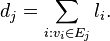
For each linearly independent linear relation there is a line in the output of the following form:

l_0 l_1 ... l_{n-1} d=l codim=c

In other words, these lines give a basis of the vector space of linear relations among the vertices. The basis is completely fixed by the order of the vertices, and the conditions that each vector, i.e. each linear relation is positive and primitive. To suppress these lines see the option -V.

Moreover, the output lines containing the information about the nef-partitions get additional data besides the standard output. This data are the degrees of the parts of the nef-partition with respect to the linear relations. Consider a codimension $r\,$ nef-partition defined by $r\,$ collections of vertices $E_0,\dots E_{r-1}$ such that every vertex is a member of some collection $E_i\,$ . The (multi)degree of the nef-partition $\{E_0,\dots,E_{r-1}\}$ with respect to the linear relation $\sum_{i=0}^{n-1} l_i\,v_i = 0$ is the vector $(d_0,\dots,d_{r-1})$ where

$d_j = \sum_{i:v_i \in E_j} l_i.$

Note that $\sum_{j=1}^r d_j = l$ , the degree of the linear relation. The degrees $(d_0,\dots,d_{r-1})$ are the degrees of the polynomials defining the complete intersection. If the codimension is 2 the output lines describing the nef-partitions take the following form

H:# [#] P:# V:#  #   (d10 d11) ... (dn0 dn1)    #sec #cpu

or if the codimension $r\,$ is bigger than 2

H:# [#] P:# V0:#  # V1:#  # ... V(r-2):#  #      (d10 ... d1(r-1)) ... (dn0 ... dn(r-1)) #sec #cpu

The additional data is (d10 d11) ... (dn0 dn1) and (d10 ... d1(r-1)) ... (dn0 ... dn(r-1)), respectively, where n is the number of linearly independent linear relations. If $d_i = (d_{i0},\dots,d_{i,r-1})$ are the degrees with respect to the i-th linear relation, then di0 = $d_{i0}\,$ , ..., di(r-1) = $d_{i,r-1}\,$ .

The following example of a codimension 2 complete intersection taken from arXiv:hep-th/0410018v2 illustrates this option

palp$ nef.x -Lv
Degrees and weights  `d1 w11 w12 ... d2 w21 w22 ...'
  or `#lines #colums' (= `PolyDim #Points' or `#Points PolyDim'):
5 1 1 1 1 1 0 0  4 0 0 0 1 1 1 1 
5 1 1 1 1 1 0 0  4 0 0 0 1 1 1 1 M:378 12 N:8 7  codim=2 #part=8
5 7 Vertices in N-lattice:
    0   -1    0    1    0    0    0
    0   -1    1    0    0    0    0
   -1    0    0    0    0    0    1
   -1    1    0    0    1    0    0
   -1    1    0    0    0    1    0
-----------------------------------
    1    1    1    1    0    0    1  d=5  codim=1
    1    0    0    0    1    1    1  d=4  codim=2
H:2 64 [-124] P:0 V:0 6   (2 3) (2 2)     1sec  0cpu
H:2 64 [-124] P:1 V:0 1 6   (3 2) (2 2)     1sec  0cpu
H:2 74 [-144] P:2 V:2 3 5   (2 3) (1 3)     1sec  0cpu
H:2 64 [-124] P:3 V:3 5 6   (2 3) (2 2)     1sec  0cpu
H:2 86 [-168] P:4 V:3 5   (1 4) (1 3)     1sec  1cpu
H:2 74 [-144] P:5 V:3 6   (2 3) (1 3)     1sec  0cpu
np=6 d:0 p:2    0sec     0cpu

The line 5 7 Vertices in N-lattice: says that the polytope has dimension 5 and is given by 7 vertices $v_0, \dots, v_{6}$ . Let $e_1,\dots, e_5$ be the standard basis of $\mathbb{R}^5$ . From the columns of the subsequent 5 by 7 array of numbers, we read off that the 7 vertices are

$v_0 = -e_3-e_4-e_5, \; v_1=-e_1-e_2.\; v_2=e_2,\; v_3 = e_1,\; v_4 = e_4,\; v_5 = e_5, \; v_6 = e_3.$ .

Note that an arbitrary basis has been chosen. There are two linearly independent linear relations:

$v_0 + v_1 + v_2 + v_3 + v_6 = 0,\quad v_0 + v_4 + v_5 + v_6 = 0$ .

The first of these linear relations has degree 5, the second has degree 4. The corresponding subpolytopes have codimension 1 and 2, respectively. The nef-partitions and their degrees are then as follows:

$0:\; E_1=\langle v_0, v_6 \rangle,\quad E_2=\langle v_1, v_2, v_3, v_4, v_5 \rangle,\qquad d_1 = (2,3),\quad d_2 = (2,2).$

$1:\; E_1=\langle v_0, v_1, v_6 \rangle,\quad E_2=\langle v_2, v_3, v_4, v_5 \rangle,\qquad d_1 = (3,2),\quad d_2 = (2,2).$

$2:\; E_1=\langle v_2, v_3, v_5 \rangle,\quad E_2=\langle v_0, v_1, v_4, v_6 \rangle,\qquad d_1 = (2,3),\quad d_2 = (1,3).$

$3:\; E_1=\langle v_3, v_5, v_6 \rangle,\quad E_2=\langle v_0, v_1, v_2, v_4 \rangle,\qquad d_1 = (2,3),\quad d_2 = (2,2).$

$4:\; E_1=\langle v_3, v_5 \rangle,\quad E_2=\langle v_0, v_1, v_2, v_4, v_6 \rangle,\qquad d_1 = (1,4),\quad d_2 = (1,3).$

$5:\; E_1=\langle v_3, v_6 \rangle,\quad E_2=\langle v_0, v_1, v_2, v_4, v_5 \rangle,\qquad d_1 = (2,3),\quad d_2 = (1,3).$

-Lp

???

-p

Computes the nef partitions without the (time-consuming) calculation of Hodge numbers.

Example: Complete intersection Calabi-Yau fourfold of codimension two discussed in arXiv:0912.3524. Important: in Global.h set POLY_Dmax=7 or higher and recompile!

Input with -p:

palp$ nef.x -p
Degrees and weights  `d1 w11 w12 ... d2 w21 w22 ...'
  or `#lines #columns' (= `PolyDim #Points' or `#Points PolyDim'):
6 3 2 1 0 0 0 0 0 0 0 0  13 6 4 0 1 0 0 0 0 0 1 1  7 3 2 0 0 1 0 0 0 0 1 0  8 3 2 0 0 0 1 0 0 1 1 0  15 6 4 0 0 0 0 1 1 1 1 1
6 3 2 1 0 0 0 0 0 0 0 0  13 6 4 0 1 0 0 0 0 0 1 1  7 3 2 0 0 1 0 0 0 0 1 0  8 3 2 0 0 0 1 0 0 1 1 0  15 6 4 0 0 0 0 1 1 1 1 1 M:4738 39 N:15 11  codim=2 #part=11
 P:0 V:0 4 7       0sec  0cpu
 P:1 V:0 2 3 5 9  11 12 13       0sec  0cpu
 P:2 V:1 5 6 8       0sec  0cpu
 P:3 V:1 6 7 8 10       0sec  0cpu
 P:4 V:0 1 7 8       0sec  0cpu
 P:5 V:0 1 4 7 8       0sec  0cpu
 P:6 V:4 5 6       0sec  0cpu
 P:7 V:4 6 7 10       0sec  0cpu
 P:9 V:5 6       0sec  0cpu
 P:10 V:6 8       0sec  0cpu
np=10 d:0 p:1    0sec     0cpu

Input without -p (note the calculation time! (32-bit system)):

palp$ nef.x
Degrees and weights  `d1 w11 w12 ... d2 w21 w22 ...'
  or `#lines #columns' (= `PolyDim #Points' or `#Points PolyDim'):
6 3 2 1 0 0 0 0 0 0 0 0  13 6 4 0 1 0 0 0 0 0 1 1  7 3 2 0 0 1 0 0 0 0 1 0  8 3 2 0 0 0 1 0 0 1 1 0  15 6 4 0 0 0 0 1 1 1 1 1 
6 3 2 1 0 0 0 0 0 0 0 0  13 6 4 0 1 0 0 0 0 0 1 1  7 3 2 0 0 1 0 0 0 0 1 0  8 3 2 0 0 0 1 0 0 1 1 0  15 6 4 0 0 0 0 1 1 1 1 1 M:4738 39 N:15 11  codim=2 #part=11
H:8 0 1113 [6774] P:0 V:0 4 7       247sec  246cpu
H:5 0 1115 [6768] P:1 V:0 2 3 5 9  11 12 13       141sec  141cpu
H:5 0 1115 [6768] P:2 V:1 5 6 8       136sec  136cpu
H:8 0 1113 [6774] P:3 V:1 6 7 8 10       183sec  182cpu
H:8 0 1113 [6774] P:4 V:0 1 7 8       203sec  202cpu
H:5 0 1115 [6768] P:5 V:0 1 4 7 8       157sec  156cpu
H:5 0 1115 [6768] P:6 V:4 5 6       190sec  189cpu
H:8 0 1113 [6774] P:7 V:4 6 7 10       226sec  225cpu
H:8 0 1113 [6774] P:9 V:5 6       246sec  246cpu
H:7 0 958 [5838] P:10 V:6 8       236sec  234cpu
np=10 d:0 p:1  236sec   234cpu

-D

This option keeps those nef partitions which are direct products of lower-dimensional nef partitions.

Example: Codimension 2 CICY in $\mathbb{P}^2\times \mathbb{P}^2$

with option -D:

palp$ nef.x -D
3 1 1 1 0 0 0 3 0 0 0 1 1 1
3 1 1 1 0 0 0  3 0 0 0 1 1 1 M:100 9 N:7 6  codim=2 #part=5
H:4 [0] h1=2 P:0 V:2 3 5   D     0sec  0cpu
H:20 [24] P:1 V:3 4 5       0sec  0cpu
H:20 [24] P:2 V:3 5       0sec  0cpu
H:20 [24] P:3 V:4 5       0sec  0cpu
np=3 d:1 p:1    0sec     0cpu

The last three nef partitions describe a K3 manifold. The first one is a $T^4=T^2\times T^2$ . The extra output triggered by -D is:

H:4 [0] h1=2 P:0 V:2 3 5   D     0sec  0cpu

$h 1 = 2$ indicates that the Hodge number $h 1,0 = 2$ . Furthermore $D$ indicates that the nef partition is a direct product.

Compare this to the output without the option -D where the first nef partition is not shown:

palp$ nef.x
3 1 1 1 0 0 0 3 0 0 0 1 1 1
3 1 1 1 0 0 0  3 0 0 0 1 1 1 M:100 9 N:7 6  codim=2 #part=5
H:20 [24] P:1 V:3 4 5       0sec  0cpu
H:20 [24] P:2 V:3 5       0sec  0cpu
H:20 [24] P:3 V:4 5       1sec  0cpu
np=3 d:1 p:1    0sec     0cpu

-P

This option also shows nef partitions corresponding to projections. If a nef partition has $k$ elements which only contain one vertex this corresponds to $k$ linear equations which set $k$ of the variables to zero. The Calabi-Yau is thus a complete intersection of codimension $k$ less.

Example: Complete intersection of codimension 2 in $\mathbb{P}^3$ :

palp$ nef.x -P
4 1 1 1 1
4 1 1 1 1 M:35 4 N:5 4  codim=2 #part=2
H:[0] P:0 V:2 3       0sec  0cpu
H:[0] P:1 V:3       0sec  0cpu
np=1 d:0 p:1    0sec     0cpu

Compared to the output without -P there is one additional line:

H:[0] P:1 V:3       0sec  0cpu

One element of the nef partition only contains the vertex labeled by $3$ . Therefore one of the equations of the complete intersections reads $x [3] = 0$ . Thus, we are left with a hypersurface in $\mathbb{P}^2$ , i.e. the cubic curve.

Example: A complete intersection of codimension 6 which is reduced to codimension 3 by projections. We use the option -c* to set the codimension and -p to suppress the calculation of the Hodge numbers. Furthermore we list the vertices using the option -Lv:

palp$ nef.x -P -c6 -p -Lv
Degrees and weights  `d1 w11 w12 ... d2 w21 w22 ...'
  or `#lines #columns' (= `PolyDim #Points' or `#Points PolyDim'):
6 1 1 1 1 1 1 0 0 0 6 1 1 1 0 0 0 1 1 1
6 1 1 1 1 1 1 0 0 0  6 1 1 1 0 0 0 1 1 1 M:5214 12 N:10 9  codim=6 #part=1
7 9 Vertices in N-lattice:
   -1    0    0    1    0    0    0    0    0
   -1    0    1    0    0    0    0    0    0
    0   -1    0    0    0    1    0    0    0
    0   -1    0    0    1    0    0    0    0
   -1    1    0    0    0    0    0    0    1
   -1    1    0    0    0    0    1    0    0
   -1    1    0    0    0    0    0    1    0
---------------------------------------------
    1    1    1    1    1    1    0    0    0  d=6  codim=2
    1    0    1    1    0    0    1    1    1  d=6  codim=2
 P:0 V0:0  V1:2  V2:3  V3:4 7  V4:5 8   (1 1 1 1 1 1) (1 1 1 1 1 1)     0sec  0cpu
np=0 d:0 p:1    0sec     0cpu

The output shows that three elements of the nef partition contain only one vertex:

 P:0 V0:0  V1:2  V2:3  V3:4 7  V4:5 8       0sec  0cpu

Therefore the variables associated to the vertices labeled by $0,2$ and $3$ can be set to zero and we are left with a complete intersection of codimension $3$ in $\mathbb{P}^2\times \mathbb{P}^2$ .

-t

The option -t gives detailed information about the calculation times of the Hodge numbers. The Hodge numbers of a complete intersection are generated by the so called stringy E-function introduced by Batyrev and Borisov in alg-geom/9509009. The combinatorial construction of the E-function involves the construction of a B-polynomial and an S-polynomial defined in alg-geom/9509009. The option -t returns the accumulated computing times of the respective polynomials.

Example: Complete intersection Calabi-Yau fourfold discussed in arXiv:0908.1784. Important: in Global.h set POLY_Dmax=7 or higher and recompile!

palp$ nef.x -t
10 3 2 0 1 1 1 1 1  6 3 2 1 0 0 0 0 0
10 3 2 0 1 1 1 1 1  6 3 2 1 0 0 0 0 0 M:2302 15 N:12 8  codim=2 #part=4
   BEGIN S-Poly     0sec  0cpu
   BEGIN B-Poly     61sec  57cpu
   BEGIN E-Poly     66sec  61cpu
H:2 30 308 [1728] P:0 V:4 5 6 7       66sec  61cpu
   BEGIN S-Poly     0sec  0cpu
   BEGIN B-Poly     92sec  83cpu
   BEGIN E-Poly     100sec  91cpu
H:5 5 448 [2736] P:1 V:5 6 7       100sec  91cpu
   BEGIN S-Poly     0sec  0cpu
   BEGIN B-Poly     152sec  138cpu
   BEGIN E-Poly     160sec  146cpu
H:5 0 567 [3480] P:2 V:6 7       160sec  146cpu
np=3 d:0 p:1    0sec     0cpu

-c*

The option -c* where * is a number $> = 1$ allows to specify the codimension of the Calabi-Yau. The default value is for the codimension is 2. Note that the calculation can become very slow for high codimensions and PALP may crash because the limits such as the number of vertices etc. set in Global.h may be exceeded.

Important: for codimension 2 or higher the parameter POLY_Dmax specifying the dimension of the polytope in Global.h needs to be changed accordingly and PALP has to be recompiled.

Example: Codimension 3 CICY in $\mathbb{P}^2\times \mathbb{P}^2$ :

palp$ nef.x -c3
Degrees and weights  `d1 w11 w12 ... d2 w21 w22 ...'
  or `#lines #columns' (= `PolyDim #Points' or `#Points PolyDim'):
3 1 1 1 0 0 0 3 0 0 0 1 1 1
3 1 1 1 0 0 0  3 0 0 0 1 1 1 M:100 9 N:7 6  codim=3 #part=7
H:[0] P:0 V0:1 3  V1:4 5       1sec  1cpu
H:[0] P:1 V0:2 3  V1:4 5       1sec  0cpu
np=1 d:1 p:5    0sec     0cpu

Also hypersurfaces are possible.

Example: Quintic in $\mathbb{P}^4$ :

palp$ nef.x -c1
Degrees and weights  `d1 w11 w12 ... d2 w21 w22 ...'
  or `#lines #columns' (= `PolyDim #Points' or `#Points PolyDim'):
5 1 1 1 1 1
5 1 1 1 1 1 M:126 5 N:6 5  codim=1 #part=1
H:1 101 [-200] P:0     math 0sec  0cpu
np=1 d:0 p:0    0sec     0cpu

Compare to that the output of poly.x:

palp$ poly.x
Degrees and weights  `d1 w11 w12 ... d2 w21 w22 ...'
  or `#lines #columns' (= `PolyDim #Points' or `#Points PolyDim'):
5 1 1 1 1 1
5 1 1 1 1 1 M:126 5 N:6 5 H:1,101 [-200]

-F*

The option -Fb yields information about possible fibrations of the toric variety associated to the given reflexive lattice polytope. The polytopes assoicated to the fibers are again restricted to be reflexive. By considering nef-partitions for the given lattice polytope this option also possible fibrations of the corresponding complete intersection Calabi-Yau manifolds by lower-dimensional complete intersection Calabi-Yau manifolds. For more details see arXiv:math/0001106v1 [math.AG] and [http:// arxiv.org/abs/hep-th/0410018 arXiv:hep-th/0410018v2].

In practice one should always use the option -Fb in conjunction with either -Lv or -Lp. The nonnegative integer b specifies the maximal codimension b of the fiber polytope. The default value for b is 2. Note that this codimension does not need to coincide with the codimension of the corresponding complete intersection Calabi-Yau fiber. See the examples below.

Besides the standard output and the output from the options -Lv or -Lp, the full information about fibration structures is listed below a second dashed line. The output takes the following form:

----------------------------------------------- #fibrations=#
    _    _    v    v    ...    p    p    p    v  cd=#  m:  #  # n: # #
                        ...
    v    p    _    v    ...    v    _    _    p  cd=#  m:  #  # n: # #

The number # in #fibrations=# specifies the number of fibrations by reflexive polytopes up to symmetry that have been found. Then each of the following lines corresponds to one of these fibrations. The points of the given polytope are labeled by either v, p or _.

v means that the corresponding point is a vertex of the fiber polytope
p means that the corresponding point is a non-vertex point of the fiber polytope
_ means that the corresponding point is not a point of the fiber polytope. These correspond to the directions in which the polytope is projected.
The nonnegative integer # in cd=# specifies the codimension of the fiber polytope
The two positive integers # # after m: specify the number of points and the number of vertices of the dual of the fiber polytope, respectively.
The two positive integers # # after n: specify the number of points and the number of vertices of the fiber polytope, respectively.

The following examples illustrate this option.

The first example is the degree 18 hypersurface in a crepant resolution of the weighted projective space $\mathbb{P}(1,1,1,6,9)$ . Since it is a hypersurface, we need to set the codimension to 1 using the option -c*.

palp$ echo "18 9 6 1 1 1" | nef.x -f -Lp -c1 -F
18 9 6 1 1 1 M:376 5 N:10 5  codim=1 #part=1
4 10  Points of Poly in N-Lattice:
    0    0   -2    3    0    2    1   -1    0    0
    0    3   -1    1    0    1    1    0    1    0
    0   -1    0    0    1    0    0    0    0    0
    1   -1    0    0    0    0    0    0    0    0
--------------------------------------------------
    1    1    9    6    1    0    0    0    0  d=18  codim=0
    0    0    2    1    0    0    1    0    0  d=4  codim=2
    0    0    1    1    0    0    0    1    0  d=3  codim=2
    0    0    3    2    0    0    0    0    1  d=6  codim=2
    0    0    1    0    0    1    0    0    0  d=2  codim=3
--------------------------------------------- #fibrations=1
    _    _    v    v    _    p    p    p    v  cd=2  m:  7  3 n: 7 3
H:2 272 [-540] P:0  (18) (4) (3) (6) (2)     0sec  0cpu
np=1 d:0 p:0    0sec     0cpu

There is only one fibration whose fiber polytope has codimension 2. Since the whole polytope has dimension 4, the fiber polytope therefore has dimension 4-2=2, and the dimension of the fiber of the associated toric variety is also 2. Since we are considering a hypersurface, i.e. a complete intersection of codimension 1, the corresponding Calabi-Yau manifold $X\,$ has dimension 4-1=3 and admits a fibration by elliptic curves since the fiber has dimension 2-1=1. We can specify the fiber even more by looking at the entries v, p and _ and comparing them to the linear relations of the same codimension as the fiber polytope above the second dashed line. We observe that the relation 0 0 3 2 0 0 0 0 1 d=6 codim=2 has precisely a zero for each point labelled by a _. Hence the fiber of the toric variety is (a crepant resolution of) the weighted projective space $\mathbb{P}(1,2,3)$ , and the fiber of $X\,$ is a degree 6 curve in this weighted projective space.

The next example is again a hypersurface, the degree 24 hypersurface in the crepant resolution of the weighted projective space $\mathbb{P}(1,1,2,8,12)$ .

palp$ echo "24 12 8 2 1 1" | nef.x -f -Lp -c1 -F
24 12 8 2 1 1 M:335 5 N:11 5  codim=1 #part=1
4 11  Points of Poly in N-Lattice:
    0    0   -2    3    0    1    2    0   -1    0    0
    2    0   -1    1    0    1    1    1    0    0    0
    1    2   -1    1    0    1    1    1    0    1    0
   -1    1    0    0    1    0    0    0    0    1    0
-------------------------------------------------------
    2    1   12    8    1    0    0    0    0    0  d=24  codim=0
    1    0    6    4    0    0    0    0    0    1  d=12  codim=1
    0    0    2    1    0    1    0    0    0    0  d=4  codim=2
    0    0    3    2    0    0    0    1    0    0  d=6  codim=2
    0    0    1    1    0    0    0    0    1    0  d=3  codim=2
    0    0    1    0    0    0    1    0    0    0  d=2  codim=3
-------------------------------------------------- #fibrations=2
    v    _    v    v    _    p    p    p    p    v  cd=1  m: 39  4 n: 9 4
    _    _    v    v    _    p    p    v    p    _  cd=2  m:  7  3 n: 7 3
H:3 243 [-480] P:0  (24) (12) (4) (6) (3) (2)     0sec  0cpu
np=1 d:0 p:0    0sec     0cpu

There a now two fibrations, one of codimension 1 and one of codimension 2.

The same considerations as in the example above show that the latter yields an elliptic fibration of the corresponding Calabi-Yau threefold $X\,$ with the same elliptic fiber.
The fiber polytope of the first fibration has dimension 4-1=3 and the dimension of the fiber of the associated toric variety is also 3. Since we are considering a complete intersection of codimension 1, the corresponding Calabi-Yau threefold $X\,$ admits a fibration by K3 surfaces since the fiber has dimension 3-1=2. By comparing the points with te labels _ and the linear relations of codimension 1 with a 0 at these points, we see that the fiber is a degree 12 hypersurface in (a crepant resolution of) the weighted projective space $\mathbb{P}(1,1,4,6)$ .
Note that the points labelled with _ of the first fibration form a subset of the points labelled with _ of the second fibration. This means that the fiber polytope of the first fibration admits itself a fibration by a reflexive lattice polytope, the fiber being the fiber polytope of the second fibration. Hence the fibrations of the corresponding Calabi-Yau threefold $X\,$ are compatible in the sense that the elliptic fibration factors through the K3 fibration.
Note that if one had specified the option -F1 instead of -F or -F2, only the first fibration would have been listed.

The next example is a complete intersection of codimension 2 with several fibrations. In order to find all fibration the argument of -F must be set to 3. This is an example where the interpretation of the fibration information depends on the choice of the nef-partition.

palp$ echo "12 4 2 2 2 1 1 0  8 4 0 0 0 1 1 2" | nef.x -f -Lp -c2 -F3
12 4 2 2 2 1 1 0  8 4 0 0 0 1 1 2 M:371 12 N:10 7  codim=2 #part=5
5 10  Points of Poly in N-Lattice:
    0    0    0    1    0   -1    0    0    0    0
    0    0    1    0    0   -1    0    0    0    0
   -1    4    0    0    0    0    0    1    2    0
    0   -1    0    0    1    0    0    0    0    0
   -1    2    0    0    0    1    1    1    1    0
--------------------------------------------------
    4    1    2    2    1    2    0    0    0  d=12  codim=0
    4    1    0    0    1    0    2    0    0  d=8  codim=2
    2    0    1    1    0    1    0    0    1  d=6  codim=1
    2    0    0    0    0    0    1    0    1  d=4  codim=3
    1    0    0    0    0    0    0    1    0  d=2  codim=4
--------------------------------------------- #fibrations=3
    v    v    _    _    v    _    v    p    p  cd=2  m: 35  4 n: 7 4
    v    _    v    v    _    v    v    p    v  cd=1  m:117  9 n: 8 6
    v    _    _    _    _    _    v    p    v  cd=3  m:  9  3 n: 5 3
H:4 58 [-108] P:1 V:0 2   (6 6) (4 4) (3 3) (2 2) (1 1)     1sec  0cpu
H:3 65 [-124] P:2 V:0 2 3   (8 4) (4 4) (4 2) (2 2) (1 1)     1sec  0cpu
H:3 83 [-160] P:3 V:3 5   (4 8) (0 8) (2 4) (0 4) (0 2)     1sec  1cpu
np=3 d:0 p:2    0sec     0cpu

Fuer cd=1 erhalten wir eine K3 Faserung. Die Fasern kann man aus der Zeile mit codim=1 und den Degrees unten ablesen, es sind P(1,1,1,1,2)[3,3], P(1,1,1,1,2)[4,2] bzw. P(1,1,1,1,2)[2,4] fuer die drei Partitionen.

Naiv wuerde man erwarten, dass man fuer cd=2 eine elliptische Faserung bekommen wuerde wie im Hyperflaechenfall oben. Dies ist richtig fuer die ersten beiden Partitionen. Die Faser liest man aus der Zeile mit codim=2 ab und erhaelt P(1,1,2,4)[4,4] in beiden Faellen. Genaueres Studium zeigt, dass die eine Grad 4 Gleichung nur den Vertex mit Gewicht 4 betrifft, die Gleichung ist also trivial, und wir koennen beides weglassen. Die Faser ist also P(1,1,2)[4].

Bei der dritten hingegen sieht man, dass das Faserpolytop vollstaendig in einer der beiden Partitionen liegt. Im Detail: Die Eintraege entsprechend V: 3 5 sind alle _, d.h. alle v sind in der Partition 0 1 2 4 6. Bei den anderen beiden Partitionen gehoeren gibt es ein v bei 0 (in der einen Partition) und ein v bei 6 (in der anderen Partition) , d.h. das Faserpolytop liegt in beiden Partitionen. Bei den ersten beiden Partitionen ist die Faser also eine Kodimension 2 CICY in einem 3d Polytop, d.h. eine elliptische Kurve, wie oben beschrieben.

Bei der dritten Partition hingegen ist die Faser eine Kodimension 1 (die Vertizes des Faserpolytops haben nur eine Partition) CICY, d.h. eine Hyperflaeche in diesem 3D Polytop, also eine K3. Die K3 ist P(1,1,2,4)[8,0] = P(1,1,2,4)[8]. Dieses Phaenomen ist in hep-th/0410018 beschrieben.

Schliesslich wuerde man fuer das Faser-Polytop mit cd=3 nur Punkte als Fasern erwarten, also gar keine Faserung. Das ist in der Tat der Fall fuer die ersten beiden Partitionen. Aber fuer die dritte liegt das Faserpolytop mit den Vertizes 0 6 8 vollstaendig in der Partition 0 1 2 4 6 7 8, d.h. wir bekommen eine elliptische Faser der Form P(1,1,2)[4].

Beachte folgendes Phaenomen, dass nur bei CICYs auftritt: Der Punkt 8 ist kein Vertex des Gesamtpolytops, aber er tritt als Vertex der Faserpolytope in cd=1 und cd=3 auf.

-y

Depending on the input the option -y returns the weight matrix or the vertices of the M-lattice polytope if there is at least one nef partition. In order to trigger the output this nef partition may also be a projection (or a direct product? - example needed). If there is no nef partition there is no output.

Depending on the input the following output is given:

if there is a nef partition:

- If the input is a weight matrix, the weight matrix is returned along with the polytope data.

- If the input is a polytope in the M-lattice or N-lattice (cf. option -N) the M-lattice polytope is returned.

if there is no nef partition

- If the input is a weight matrix, the weight matrix is returned without further information about the polytope.

- If the input is a polytope there is no output.

Example: Codimension 2 complete intersection in $\mathbb{P}^3$ , input is the weight matrix:

palp$ nef.x -y
Degrees and weights  `d1 w11 w12 ... d2 w21 w22 ...'
  or `#lines #columns' (= `PolyDim #Points' or `#Points PolyDim'):
4 1 1 1 1
4 1 1 1 1 M:35 4 N:5 4  codim=2 #part=2

Example: Codimension 2 complete intersection in $\mathbb{P}^3$ , input is the N-lattice polytope:

palp$ nef.x -y -N
Degrees and weights  `d1 w11 w12 ... d2 w21 w22 ...'
  or `#lines #columns' (= `PolyDim #Points' or `#Points PolyDim'):
3 4
Type the 12 coordinates as dim=3 lines with #pts=4 columns:
-1    0    0    1
-1    0    1    0
-1    1    0    0    
3 4 Vertices of Poly in M-lattice:  M:35 4 N:5 4  codim=2 #part=2
   -1   -1   -1    3
   -1   -1    3   -1
   -1    3   -1   -1

Example: Codimension 2 complete intersection in $\mathbb{P}^3$ , input is the M-lattice polytope:

palp$ nef.x -y
Degrees and weights  `d1 w11 w12 ... d2 w21 w22 ...'
  or `#lines #columns' (= `PolyDim #Points' or `#Points PolyDim'):
3 4
Type the 12 coordinates as dim=3 lines with #pts=4 columns:
   -1   -1   -1    3
   -1   -1    3   -1
   -1    3   -1   -1
3 4 Vertices of Poly in M-lattice:  M:35 4 N:5 4  codim=2 #part=2
   -1   -1   -1    3
   -1   -1    3   -1
   -1    3   -1   -1

Example without a nef partition, input is the weight matrix:

palp$ nef.x -y
Degrees and weights  `d1 w11 w12 ... d2 w21 w22 ...'
  or `#lines #columns' (= `PolyDim #Points' or `#Points PolyDim'):
6 3 2 1 0 0 6 3 0 0 2 1
6 3 2 1 0 0  6 3 0 0 2 1

Example without a nef partition, input is the N-lattice polytope:

palp$ nef.x -y -N
Degrees and weights  `d1 w11 w12 ... d2 w21 w22 ...'
  or `#lines #columns' (= `PolyDim #Points' or `#Points PolyDim'):
3 5
Type the 15 coordinates as dim=3 lines with #pts=5 columns:
 0    0   -1    2    0
-2    3    3    0    0
-1    1    1    1    1
Degrees and weights  `d1 w11 w12 ... d2 w21 w22 ...'
  or `#lines #columns' (= `PolyDim #Points' or `#Points PolyDim'):

The same holds if an M-lattice polytope is entered.

-S

The option -S gives information about the number of points in the Gorenstein cone and its dual (cf. options -g* and -d*) for every nef partition which is not a direct product or a projection. It counts the number of points and interior points at distance $1,\ldots,d$ from the origin, where $d$ is the dimension of the polytope. These data enter the calculation of the Hodge numbers using the stringy E-function, to be precise in the calculation of the S-polynomial (hence the name -S), as described in alg-geom/9509009.

Example: Complete intersection of codimension 2 in $\mathbb{P}^4$

palp$ nef.x -S
Degrees and weights  `d1 w11 w12 ... d2 w21 w22 ...'
  or `#lines #columns' (= `PolyDim #Points' or `#Points PolyDim'):
4 1 1 1 1
4 1 1 1 1 M:35 4 N:5 4  codim=2 #part=2


#points in largest cone:
layer:  1 #p:        6 #ip:        0
layer:  2 #p:       21 #ip:        1
layer:  3 #p:       56 #ip:        6


#points in largest cone:
layer:  1 #p:       20 #ip:        0
layer:  2 #p:      105 #ip:        1
layer:  3 #p:      336 #ip:       20
H:[0] P:0 V:2 3       0sec  0cpu
np=1 d:0 p:1    0sec     0cpu

One of the two nef partitions is a projection and is not analyzed. The output for the remaining nef partition has two blocks:

The first block counts the numbers of points (after $\#p$ ) and interior points (after $\#ip$ ) of the Gorenstein cone in the N-lattice at distances $1,2,3$ form the origin. One can check that the number of points at layer $1$ indeed coincides with the number of points in the output of the option -g2.
The second block gives the same information for the dual Gorenstein cone in the M-lattice. The output of the option -d2 coincides with the number of points at layer $1$ .

-T

???

-s

The option -s also includes nef partitions in the output which are related bt to symmetries of the weight matrix. Note that the option -s does not print all possible nef partitions as those corresponding to projections (cf. option -P) or direct products (cf. option -D) are left out.

Expample: Complete intersection of codimension 2 in $\mathbb{P}^2\times\mathbb{P}^2$ . We add the option -Lv in order to print the vertices and the weight matrix.

palp$ nef.x -s -Lv
Degrees and weights  `d1 w11 w12 ... d2 w21 w22 ...'
  or `#lines #columns' (= `PolyDim #Points' or `#Points PolyDim'):
3 1 1 1 0 0 0 3 0 0 0 1 1 1
3 1 1 1 0 0 0  3 0 0 0 1 1 1 M:100 9 N:7 6  codim=2 #part=31
4 6 Vertices in N-lattice:
    0    0    0    1    0   -1
    0    0    1    0    0   -1
   -1    0    0    0    1    0
   -1    1    0    0    0    0
------------------------------
    1    1    0    0    1    0  d=3  codim=2
    0    0    1    1    0    1  d=3  codim=2
H:20 [24] P:2 V:4 5   (1 2) (1 2)     0sec  0cpu
H:20 [24] P:4 V:0 5   (1 2) (1 2)     0sec  0cpu
H:20 [24] P:5 V:0 4   (2 1) (0 3)     0sec  0cpu
H:20 [24] P:6 V:0 4 5   (2 1) (1 2)     0sec  0cpu
H:20 [24] P:8 V:1 5   (1 2) (1 2)     1sec  0cpu
H:20 [24] P:9 V:1 4   (2 1) (0 3)     0sec  0cpu
H:20 [24] P:10 V:1 4 5   (2 1) (1 2)     0sec  0cpu
H:20 [24] P:11 V:0 1   (2 1) (0 3)     0sec  0cpu
H:20 [24] P:12 V:0 1 5   (2 1) (1 2)     0sec  0cpu
H:20 [24] P:14 V:2 3   (0 3) (2 1)     0sec  0cpu
H:20 [24] P:16 V:2 5   (0 3) (2 1)     0sec  0cpu
H:20 [24] P:17 V:2 4   (1 2) (1 2)     0sec  0cpu
H:20 [24] P:18 V:2 4 5   (1 2) (2 1)     0sec  0cpu
H:20 [24] P:19 V:0 2   (1 2) (1 2)     0sec  0cpu
H:20 [24] P:20 V:0 2 5   (1 2) (2 1)     1sec  0cpu
H:20 [24] P:21 V:0 2 4   (2 1) (1 2)     0sec  0cpu
H:20 [24] P:22 V:1 3   (1 2) (1 2)     0sec  0cpu
H:20 [24] P:23 V:1 2   (1 2) (1 2)     0sec  0cpu
H:20 [24] P:24 V:1 2 5   (1 2) (2 1)     0sec  0cpu
H:20 [24] P:25 V:1 2 4   (2 1) (1 2)     0sec  0cpu
H:20 [24] P:26 V:0 3   (1 2) (1 2)     0sec  0cpu
H:20 [24] P:27 V:0 1 2   (2 1) (1 2)     0sec  0cpu
H:20 [24] P:28 V:3 4   (1 2) (1 2)     1sec  0cpu
H:20 [24] P:29 V:3 5   (0 3) (2 1)     0sec  0cpu
np=24 d:1 p:6    0sec     0cpu

Note that the weight matrix is symmetric under permutations of the vertices labeled by $0,1,4$ and those labeled by $2,3,5$ . Furthermore there only exist three pairs of degrees of the complete intersection (up to exchange within a pair): ${(1,2),(1,2)},{(0,3),(2,1)},{(1,2),(2,1)}$ . Therefore we conclude that there are only three inequivalent nef partitions. This is indeed confirmed by calling nef without the option -s:

palp$ nef.x -Lv
Degrees and weights  `d1 w11 w12 ... d2 w21 w22 ...'
  or `#lines #columns' (= `PolyDim #Points' or `#Points PolyDim'):
3 1 1 1 0 0 0 3 0 0 0 1 1 1
3 1 1 1 0 0 0  3 0 0 0 1 1 1 M:100 9 N:7 6  codim=2 #part=5
4 6 Vertices in N-lattice:
    0    0    0    1    0   -1
    0    0    1    0    0   -1
   -1    0    0    0    1    0
   -1    1    0    0    0    0
------------------------------
    1    1    0    0    1    0  d=3  codim=2
    0    0    1    1    0    1  d=3  codim=2
H:20 [24] P:1 V:3 4 5   (1 2) (2 1)     0sec  0cpu
H:20 [24] P:2 V:3 5   (0 3) (2 1)     0sec  0cpu
H:20 [24] P:3 V:4 5   (1 2) (1 2)     0sec  0cpu
np=3 d:1 p:1    0sec     0cpu

-n

The option -n prints the points of the polytope in the N-lattice only if there is at least one nef partition which does not correspond to a projection or a direct product. If there is no nef partition the polytope is not printed. In addition the number of nef partitions, the codimension and the number of points and vertices in the M- and N-lattice polytope is printed.

Example with nef partition: Codimension 2 complete intersection in $\mathbb{P}^3$

palp$ nef.x -n
Degrees and weights  `d1 w11 w12 ... d2 w21 w22 ...'
  or `#lines #columns' (= `PolyDim #Points' or `#Points PolyDim'):
4 1 1 1 1
4 1 1 1 1 M:35 4 N:5 4  codim=2 #part=2
3 5  Points of Poly in N-Lattice:
   -1    0    0    1    0
   -1    0    1    0    0
   -1    1    0    0    0

Example without a nef partition:

palp$ nef.x -n
Degrees and weights  `d1 w11 w12 ... d2 w21 w22 ...'
  or `#lines #columns' (= `PolyDim #Points' or `#Points PolyDim'):
6 3 2 1 0 0 6 3 0 0 2 1
6 3 2 1 0 0  6 3 0 0 2 1 M:21 5 N:12 5  codim=2 #part=0

Here the N-lattice polytope is not printed.

Example: no output of the polytope if there is only a nef partition corresponding to a projection:

Degrees and weights  `d1 w11 w12 ... d2 w21 w22 ...'
  or `#lines #columns' (= `PolyDim #Points' or `#Points PolyDim'):
6 3 2 1 0 0 3 1 0 0 1 1
6 3 2 1 0 0  3 1 0 0 1 1 M:24 6 N:9 5  codim=2 #part=1

We can use the option -P to check that the nef partition corresponding a projection:

palp$ nef.x -P
Degrees and weights  `d1 w11 w12 ... d2 w21 w22 ...'
  or `#lines #columns' (= `PolyDim #Points' or `#Points PolyDim'):
6 3 2 1 0 0 3 1 0 0 1 1
6 3 2 1 0 0  3 1 0 0 1 1 M:24 6 N:9 5  codim=2 #part=1
H:[0] P:0 V:4  DP      0sec  0cpu
np=0 d:0 p:1    0sec     0cpu

???: this is a projection but there is an output DP - what does that mean?

-v

The option -v prints the size of the matrix of vertices, the number of points and the vertices of the polytope that has been entered (M-lattice or N-lattice, depending on the input!). If the input is the weight matrix the M-lattice polytope is analyzed. The output is printed in a single line with the character $E$ as seperator. Furthermore one can limit the output to polytopes whose number of points is limited to a lower and an upper bound:

-v -u#, where # is an integer $> 0$ , only gives output if the polytope has at most # points. The default value is the parameter POINT_Nmax which fixes the maximal number of points of a polytope at compilation.
-v -l#, where # is an integer $> 0$ , only gives output if the polytope has at least # points.The default value is 0.

After closing the program a summary is printed. It contains information on how many of the polytopes examined satisfy the bounds and how many polutopes with # of points have been found.

Example: Complete intersections of codimesnion 2 in $\mathbb{P}^3$ and $\mathbb{P}^2\times\mathbb{P}^2$ with the weight matrices as input and without bounds.

palp$ nef.x -v
Degrees and weights  `d1 w11 w12 ... d2 w21 w22 ...'
  or `#lines #columns' (= `PolyDim #Points' or `#Points PolyDim'):
4 1 1 1 1
3 4 P:35 E   -1    3   -1   -1E   -1   -1    3   -1E   -1   -1   -1    3
Degrees and weights  `d1 w11 w12 ... d2 w21 w22 ...'
  or `#lines #columns' (= `PolyDim #Points' or `#Points PolyDim'):
3 1 1 1 0 0 0 3 0 0 0 1 1 1
4 9 P:100 E   -1    2   -1   -1    2   -1   -1    2   -1E   -1   -1    2   -1   -1    2   -1   -1    2E   -1   -1   -1    2    2    2   -1   -1   -1E   -1   -1   -1   -1   -1   -1    2    2    2
Degrees and weights  `d1 w11 w12 ... d2 w21 w22 ...'
  or `#lines #columns' (= `PolyDim #Points' or `#Points PolyDim'):



2  of  2

  35#    1
 100#    1

Since we have entered a weight matrix the M-lattice polytope is analyzed. Let us discuss the first line of output:

3 4 P:35 E   -1    3   -1   -1E   -1   -1    3   -1E   -1   -1   -1    3

The first two numbers indicate the number of rows and columns of the matrix of vertices in the M-lattice polytope. P:35 indicates that the M-lattice polytope has 35 points. The vertices of the M-lattice polytope are then written in one line with the seperator E. The output of the second example is analogous. After we quit PALP by hitteng enter without input the following output is given:

This means that 2 out of the 2 polytopes analyzed satisfy the bounds and that there is one polytope with 35 points and one with 100.

Example: Same example as above but with the upper bound for the number of points set to 50:

palp$ nef.x -v -u50
Degrees and weights  `d1 w11 w12 ... d2 w21 w22 ...'
  or `#lines #columns' (= `PolyDim #Points' or `#Points PolyDim'):
4 1 1 1 1
3 4 P:35 E   -1    3   -1   -1E   -1   -1    3   -1E   -1   -1   -1    3
Degrees and weights  `d1 w11 w12 ... d2 w21 w22 ...'
  or `#lines #columns' (= `PolyDim #Points' or `#Points PolyDim'):
3 1 1 1 0 0 0 3 0 0 0 1 1 1
Degrees and weights  `d1 w11 w12 ... d2 w21 w22 ...'
  or `#lines #columns' (= `PolyDim #Points' or `#Points PolyDim'):



1  of  2

  35#    1

Now the second polytope exceeds the upper bound for the points as it has 100 points (cf. previous example). There is no output for the second polytope and the summary indicates that only one of the two polytopes analyzed satisfies the bounds.

Example: same example as above but now we enter the N-lattice polytope and search for polytopes which have at least 7 points in the N-lattice.

Degrees and weights  `d1 w11 w12 ... d2 w21 w22 ...'
  or `#lines #columns' (= `PolyDim #Points' or `#Points PolyDim'):
3 4
Type the 12 coordinates as dim=3 lines with #pts=4 columns:
   -1    0    0    1
   -1    0    1    0
   -1    1    0    0
Degrees and weights  `d1 w11 w12 ... d2 w21 w22 ...'
  or `#lines #columns' (= `PolyDim #Points' or `#Points PolyDim'):
4 6
Type the 24 coordinates as dim=4 lines with #pts=6 columns:
    0    0    0    1    0   -1
    0    0    1    0    0   -1
   -1    0    0    0    1    0
   -1    1    0    0    0    0
4 6 P:7 E    0    0    0    1    0   -1E    0    0    1    0    0   -1E   -1    0    0    0    1    0E   -1    1    0    0    0    0
Degrees and weights  `d1 w11 w12 ... d2 w21 w22 ...'
  or `#lines #columns' (= `PolyDim #Points' or `#Points PolyDim'):



1  of  2

   7#    1

There is no output for the first polytope because it has less than 7 vertices. As one can check using option -Lp the N-lattice polytope has only 5 points. There is output for the second polytope since it has seven points and therefore satisfies the bound.

-m

The option -m returns a Minkowski sum decomposition of codimension 2 $\nabla=\nabla_1 + \nabla_2$ with specified degrees $d_1, d_2\,$ . The input data is a single weight vector which will be part of a combined weight system describing a polytope $\nabla\,$ in the lattice $N\,$ , and a pair of degrees $(d_1,d_2)\,$ that add up to the degree $d\,$ of the weight vector. The following example taken from hep-th/0410018 illustrates this option

palp$ nef.x -m
type degrees and weights [d  w1 w2 ... wk d=d_1 d_2]: 14 1 1 1 1 4 6 d=2 12
14 1 1 1 1 4 6 d=2 12 M:1270 12 N:11 7  codim=2 #part=2
 d=12 2H:3 243 [-480] P:0 V:3 5       6sec  6cpu
np=1 d:0 p:1    0sec     0cpu

We consider the weighted projective space $\mathbb{P}(1,1,1,1,4,6)$ specified by the weight vector 14 1 1 1 1 4 6 of degree $d=14\,$ . We are looking for a combined weight system describing a polytope $\nabla\,$ and decomposition of $\nabla\,$ into a Minkowski sum $\nabla=\nabla_1 + \nabla_2$ such that the degrees of the parts $E_1, E_2\,$ of the corresponding nef-partition are $d_1=2\,$ and $d_2=12\,$ , respectively, with $d_1+d_2=d=14\,$ . The output indeed yields a polytope $\nabla\,$ and such a nef-partition. To understand the output in more detail we repeat the computation with the option -Lv:

esche$ nef.x -Lv -m
type degrees and weights [d  w1 w2 ... wk d=d_1 d_2]: 14 1 1 1 1 4 6  d=2 12
14 1 1 1 1 4 6 d=2 12 M:1270 12 N:11 7  codim=2 #part=2
5 7 Vertices in N-lattice:
    0   -1    0    0    0    1    0
    0   -1    1    0    0    0    0
    0   -1    0    1    0    0    0
    0   -4    0    0    1    0   -2
    1   -6    0    0    0    0   -3
-----------------------------------
    6    1    1    1    4    1    0  d=14  codim=0
    3    0    0    0    2    0    1  d=6  codim=3
 d=12 2H:3 243 [-480] P:0 V:3 5   (2 12) (0 6)     7sec  6cpu
np=1 d:0 p:1    0sec     0cpu

Let $e_1,\dots, e_5$ be the standard basis of $\mathbb{R}^5$ . From the columns of the subsequent 5 by 7 array of numbers, we read off that the 7 vertices are

$v_0 = e_5, \; v_1=-e_1-e_2-e_3-4e_4-6e_5.\; v_2=e_2,\; v_3 = e_3,\; v_4 = e_4,\; v_5 = e_1, \; v_6 = -2e_4-3e_5.$ .

There are two linearly independent linear relations:

$6v_0 + v_1 + v_2 + v_3 + 4v_3 + v_5 = 0,\quad 3v_0 + 2v_4 + v_6 = 0$ ,

whose degrees are 14 and 6, respectively. The nef-partition of $\nabla\,$ and its degrees are then as follows:

$0:\; E_1=\langle v_3, v_5 \rangle,\quad E_2=\langle v_0, v_1, v_2, v_4, v_6 \rangle,\qquad d_1 = (2,12),\quad d_2 = (0,6).$

The Hodge numbers and the Euler number of the corresponding Calabi-Yau threefold $X\,$ are $h^{1,1}(X) = 3, h^{2,1}(X) =243, \chi(X) = -480\,$ . We observe that the polytope $\nabla\,$ is specified by a combined weight system containing the weight vector 6 3 2 0 0 0 0 1 besides the given weight vector 14 6 4 1 1 1 1. Because of this, the Calabi-Yau 3-fold $X\,$ is, however, not a complete intersection of codimension 2 in the weighted projective space $\mathbb{P}(1,1,1,1,4,6)$ since the corresponding polytope only admits a nef-partition with degree (8,6) and not (2,12) as the following computation shows

palp$ nef.x -Lv
Degrees and weights  `d1 w11 w12 ... d2 w21 w22 ...'
  or `#lines #colums' (= `PolyDim #Points' or `#Points PolyDim'):
14 1 1 1 1 4 6
14 1 1 1 1 4 6 M:1271 13 N:10 8  codim=2 #part=2
5 8 Vertices in N-lattice:
    0   -1    0    0    0    1    0    0
    0   -1    1    0    0    0    0    0
    0   -1    0    1    0    0    0    0
    0   -4    0    0    1    0   -1   -1
    1   -6    0    0    0    0   -1   -2
----------------------------------------
    6    1    1    1    4    1    0    0  d=14  codim=0
    1    0    0    0    1    0    1    0  d=3  codim=3
    2    0    0    0    1    0    0    1  d=4  codim=3
H:1 149 [-296] P:1 V:3 4 5 7  8   (6 8) (1 2) (2 2)     2sec  1cpu
np=1 d:0 p:1    2sec     1cpu

-R

The option -R prints the vertices of the polytope in the N-lattice if it is not reflexive.

Example: We enter the weight matrix of a polytope which is not reflexive:

palp$ nef.x -R
Degrees and weights  `d1 w11 w12 ... d2 w21 w22 ...'
  or `#lines #columns' (= `PolyDim #Points' or `#Points PolyDim'):
6 3 2 1 0 0 5 0 0 1 1 3
3 4  Vertices of P:
   -1    1    0    0
    0    1   -1    1
   -1    0    0    0

The same output is given if we enter the N-lattice polytope itself. Without the option -R there is not output if the polytope is not reflexive:

palp$ nef.x
Degrees and weights  `d1 w11 w12 ... d2 w21 w22 ...'
  or `#lines #columns' (= `PolyDim #Points' or `#Points PolyDim'):
6 3 2 1 0 0 5 0 0 1 1 3
Degrees and weights  `d1 w11 w12 ... d2 w21 w22 ...'
  or `#lines #columns' (= `PolyDim #Points' or `#Points PolyDim'):

-V

???

-Q

???

-g*

???

-d*

???

Strategy for future versions

Should we keep both help screens, or try to get everything into 'nef.x -h'?

It would be good to have a documentation of the header file Nef.h: just type whatever information you can supply into the following listing, in the standard ('/* ... */') C comment format.

#define Nef_Max 	500000
#define NP_Max          500000
#define W_Nmax (POLY_Dmax+1)
#define MAXSTRING	100

#undef	WRITE_CWS
#define	WRITE_CWS

#define Pos_Max   (POLY_Dmax + 2)
#define FIB_Nmax        10*EQUA_Nmax
#define FIB_POINT_Nmax  VERT_Nmax

typedef struct {
  Long W[FIB_Nmax][FIB_POINT_Nmax];
  Long VM[FIB_POINT_Nmax][POLY_Dmax];
  int nw;
  int nv;
  int d;
  int Wmax;
} LInfo;

struct Poset_Element {
  int num, dim;
};

struct Interval {
  int min, max;
};

typedef struct Interval Interval;

typedef struct {
  struct Interval *L;
  int n;
} Interval_List;

typedef struct Poset_Element Poset_Element;

typedef struct {
  struct Poset_Element x, y;
} Poset;

typedef struct {
  struct Poset_Element *L;
  int n;
} Poset_Element_List;

typedef struct {
  int nface[Pos_Max];
  int dim;
  INCI edge[Pos_Max][FACE_Nmax];
} Cone;

typedef struct {
  Long S[2*Pos_Max];
} SPoly;

typedef struct {
  Long B[Pos_Max][Pos_Max];
} BPoly;

typedef struct {
  int E[4*(Pos_Max)][4*(Pos_Max)];
} EPoly;

typedef struct {
    Long x[POINT_Nmax][W_Nmax];
    int N, np;
} AmbiPointList;

typedef struct {
  int n;
  int nv;
  int codim;
  int S[Nef_Max][VERT_Nmax];
  int DirProduct[Nef_Max];
  int Proj[Nef_Max];
  int DProj[Nef_Max];
} PartList;

typedef struct {
  int n;
  int nv;
  int S[Nef_Max][VERT_Nmax];
} Part;

typedef struct {
  int n, y, w, p, t, S, Lv, Lp, N, u, d, g, VP, B, T, H, dd, gd, 
	noconvex, Msum, Sym, V, Rv, Test, Sort, Dir, Proj, f;		
} Flags;

typedef struct {
	int noconvex, Sym, Test, Sort;		
} NEF_Flags;

struct Vector {
  Long x[POLY_Dmax];
};

typedef struct Vector Vector ;

typedef struct {
  struct Vector *L;
  int n;
  Long np, NP_max;						} DYN_PPL;

void part_nef(PolyPointList *, VertexNumList *, EqList *, PartList *,
	      int *, NEF_Flags *);

void Make_E_Poly(FILE *, CWS *, PolyPointList *, VertexNumList *, EqList *,
		 int *, Flags *, int *);

void Mink_WPCICY(AmbiPointList * _AP_1, AmbiPointList * _AP_2,
		 AmbiPointList * _AP);

int  IsDigit(char);

int  IntSqrt(int q);

void Die(char *);

void Print_CWS_Zinfo(CWS *);

Documentation on nef.x

Contents

Standard output

Global parameters and limitations

Help screens

The options in detail

-N

-H

-Lv

-Lp

-p

-D

-P

-t

-c*

-F*

-y

-S

-T

-s

-n

-v

-m

-R

-V

-Q

-g*

-d*

Strategy for future versions

Personal tools

Namespaces

Variants

Views

Actions

Search

Navigation

Tools